Impact of CO2 on climate overestimated (substantially)
due to 66-year cycle & El Nino
September 7, 2019 - Author: Martijn van Mensvoort | ![]() Nederlandse versie (original source) |
Nederlandse versie (original source) | ![]() English version
English version
As early as 2004 the scientific literature recognizes that an extension of the definition for the climate from "minimum 30 years" to "minimum 50 years" is necessary because of the natural variability1. Since at least 2012, Dutch KNMI researchers have publicly acknowledged that a 30-year period is too short for studying weather extremes in the context of climate change2,3.
This article describes why a doubling to at least 60 years for the described duration in the definition of climate is desirable; this finding is based on the impact of the ENSO cycle + a 66-year cycle in the HadCRUT4 temperature series. The 'satellite era' only started 40 years ago in 1979; the question now arises as to whether technology may even become an obstacle to actively avoiding overestimating both trends in global warming and the impact of CO2. For the time being, the old paradigm in the definition of the climate concerning the duration of "at least 30 years" seems to indicate that within this branch of science a 'consensus' is being used based on outdated principles. This report demonstrates how the structural impact of global warming is being overestimated by the IPCC by about a factor of 2 due to the use of an approach based on a too short analysis period.
In November 2018, the KNMI described that the extremely hot years of 2015 and 2016 were largely caused by the internal variability of the climate through the emergence of the "strong El Nino"4. According to NASA, the contribution of the 'super El Nino' to the average temperature worldwide for the year 2016 was approximately 0.16°C 5. The El Nino effect causes a net cooling of the ocean system6 and is characterized by the release of large amounts of heat and CO2 in the atmosphere7. The El Nino Southern Oscillation [ENSO] also appears to have a major impact on the annual growth of CO2 in the atmosphere8; experts have estimated that the 'super El Nino' in 2016 contributed 25% of the growth of CO2 in the atmosphere9. In a broader context, Henry's law10 describes that the warming of the ocean water itself has contributed close to ~15%11 to the growth of CO2 in the atmosphere. Moreover, it has very recently become clear that in recent decades the ocean has also been responsible for up to 40% of the variability of CO2 in the atmosphere; climate models, on the other hand, assume that variability is mainly due to vegetation on the mainland12.
An earlier report in june 2019 demonstrates on the basis of the HadCRUT4 temperature series that 'global warming' is overestimated if the natural variability related to a 70-year cycle in the ocean system is not taken into account. This new report shows below that the multidecadal cycle is featured with a length of 66 years. A comparison between the 1970s, 1990s and 2010s shows that the assumed acceleration in global warming can almost entirely be attributed to the 66-year cycle. The 66-year cycle + the ENSO cycle combined appears to be responsible for more than 81% of the acceleration of the warming based on the 30-year average since the 1970s, and for more than 69% compared to the 1990s. Both natural cycles combined also largely explain the correlation between CO2 and temperature in the 21st century; 'super El Ninos' play a major role in this. This results in an overestimation of the impact of global atmospheric CO2 as well; this also applies to the acceleration with regard to the warming of the north pole.
After removal of the 66-year cycle (+ the ENSO cycle), an upwardly directed trend channel remains with an average temperature rise of approximately +0.09°C per decade that has now lasted about 70-90 years. This concerns less than half the expectation of +0.20°C per decade that the IPCC uses for the coming decades. Also, a projection has been made for the year 2100 from which it appears that based on the trend channel a temperature rise of +0.2°C to +0.9°C compared to the record year 2016 can be taken into account. A mix of factors plays a role in the emergence of the trend channel, such as: the growth of the world population, less use of sulphates (aerosols), changes in land use, use of greenhouse gases, and possibly a natural cycle of 200+ years (in the scientific literature this very long cycle is known as the Suess/de Vries cycle, which is related to the sunspots cycle). Since the 2nd half of the 1960s, a slight increase in 'total solar radiation' has had a small share in the creation of the trend channel.
An overestimation of the temperature by a factor of 2 due to natural variability can possibly imply that the impact of CO2 and other greenhouse gases is also overestimated by the IPCC with an impact of the same order.
TIP: an impression for the impact of the three natural cycles is shown in figure 13.
CONTENTS
• I - A 66 year cycle with an upward and downward phase of 33 years
• II - Warming on top of cycle shows stable trend channel
• III - Projection for the year 2100: 0.2-0.9°C on top of record year 2016
• IV - Annual growth CO2 correlates highly with ENSO cycle
• V - 21st century: correlation temperature-CO2 based on 66-year cycle & super El Nino
• VI - 21st century: warming rate 69% lower after removal of 66-year cycle & El Nino
• VII - 30-year average: acceleration in warming almost fully explained by 66-year cycle
• VIII - Four characteristics of the 66-year cycle
• IX - Five characteristics of the warming on top of the 66-year cycle
• X - 66-year cycle may have a cosmic origin
• XI - Is the definition of 'climate' outdated?
• XII - Discussion & conclusion
(Data: Excel file)
NOTE: In the run-up to the conclusion, a total of 3 different perspectives are explored:
sections II to V are based on the first perspective and sections VI & VII contain all three perspectives;
figure 14 shows all 3 perspectives compared to the 30-year average of the HadCRUT4 temperature series.
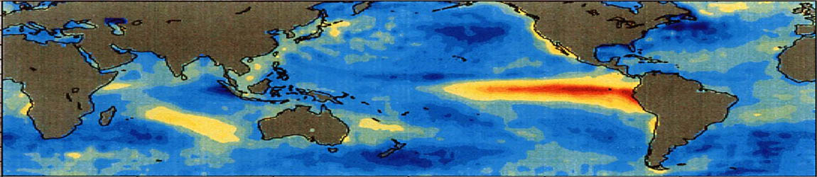
VIDEO: This is how El Nino works (source: NOAA)
El Nino relates to the upward phase of the ENSO cycle; this results in exceptional changes in the climate system. La Nina relates to the downward phase and is accompanied by a reinforcement of normal circumstances.
I - A 66 year cycle with an upward and downward phase of 33 years
Figure 1 shows the development of the annual temperature anomaly worldwide according to the British HadCRUT4 series (reference period: 1961-1990). The exact length of the multidecadal cycle is difficult to determine in this graph; cause: in the perspective of the individual years, both the upward and downward phase shows a variable length in terms of the peak and bottom years.
At the level of the decades, the graph shows a cycle of 7 decades; the average duration of two oscillations based on peak and bottom years is approximately 69 years. However, as a result of the temperature rise in recent decades, the cycle in these perspectives probably seems a bit longer than it actually is.
Based on the hypothesis that humans may be partly responsible for global warming, it seems likely that the exact duration of the multidecadal cycle may be less reliable in the perspective of temperature trends in recent decades. Moreover, the course of the 66-year cycle is also masked by the ENSO cycle.
Further investigation shows: after the separation of the multidecadal cycle and the warming on top of the cycle, a full oscillation is found that has a length of exactly 33 years in both the upward phase and in the downward phase. This results in the conclusion that the multidecadal cycle has an approximate total duration of 66 years. Section VI describes that the 66-year cycle is also found after removal of the ENSO cycle.
The 66-year cycle is also found in the previously used calculation method in june 2019 based on 7 decades. However, this is a direct consequence of the calculation method used - where the cycle is described on the basis of a comparison with the temperature trend in previous years. With the previously used 70-year cycle, the peak and bottom years are found 4 years later compared to the result based on the 66-year cycle. When a longer (or shorter) cycle length is used, the peaks and troughs shift according the amount of extra (or less) years but the distance between them remains unchanged.
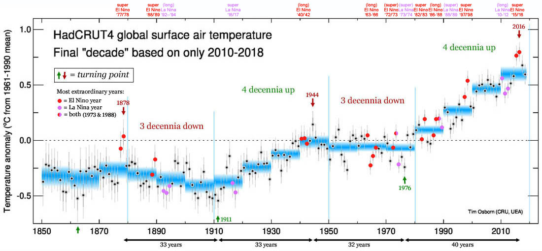
Figure 1: The HadCRUT4 temperature series shown with the strongest El Nino & La Nina years.
Based on the Ensemble Ocean Nino Index [EONI] (this is a variant of the El Nino 3.4 index), figure 1 shows the 'super El Ninos' and 'super La Ninas' plus the years in which there is a combination of both a 'strong' and 'moderate' ENSO occurrence with a concatenated duration of at least 3 years. For the period from 1850 this results in 9 El Nino periods and 5 La Nina periods. Section V describes that the 'super El Ninos' play a significant role in the rise of both the temperature and the CO2 in the atmosphere.
II - Warming on top of cycle shows stable trend channel
In Figure 2, the HadCRUT4 temperature series is split into the 66-year cycle (= the oscillating movement) and the warming on top of the cycle (= the upward-directed trend channel; the external boundaries are determined on the basis of a visual analysis and the central trend on the basis of of the average of the raised). For each individual year, the sum of the two graphs in figure 2 corresponds to the HadCRUT4 value in figure 1.
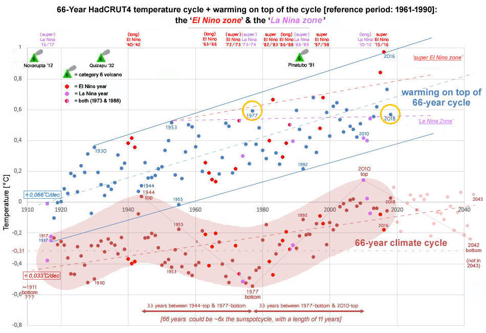
Figure 2: The 66-year cycle (the light brown band is only indicative for it's probable course) + the warming on top of the cycle; the sum of both produces the values in the HadCRUT4 temperature series.
NOTE: In figure 2 the values of the 66-year cycle for individual years are based on the annual temperature in the HadCRUT4 series 66 years earlier [= T66]. The midpoint value of -0.313°C concerns the difference between the reference period 1961-1990 on which the HadCRUT4 is based compared to the reference period 1850-1900 (which is representative of the beginning of the industrial revolution). If the reference period 1850-1900 would have been used, the midpoint of the cycle should coincide with the zero line.
For the 66-year cycle & the warming on top of the cycle applies respectively:
T66 in year X (= brown dots figure 2) = HadCRUT4 in year X-66
Warming on top of T66 in year X (= blue dots figure 2) = HadCRUT4 - T66 in year X
Important: in figure 2 the 66-year cycle shows a small upward slope with an increase of + 0.033°C per decade. However, the cycle should show a flat course; it is therefore desirable (necessary) to use a correction to remove the slope from the 66-year cycle and move it to the warming on top of the cycle. The result of this correction is shown in figure 3, where the slope of the corrected warming on top of the cycle [= Topw] has become +0.099°C per decade.
In the corrected 66-year cycle in figure 3 [= T cycle] the slope has disappeared completely after a correction that has been made with the following 2 formulas that have been applied to the HadCRUT4 temperature series [=T]:
Corrected 66-year cycle:
Tcycle (= brown dots in figure 3) = T66 + ((2047-year)*0,0033)
Corrected warming on top of 66-year cycle:
Topw (= blue dots figure 3) = T - Tcycle
The corrected 66-year cycle approximates the value zero for the period 1916-2018 for both the average value and the correlation with CO2. As a check, it has been established that for the period 1944-2010 (where symmetry is found around the low point of the corrected 66-year cycle in the year 1977) the average value also approximates zero; the correlation with CO2 is a bit higher but not significant for this period (it is not desirable for the cycle to have a significant correlation with CO2, so this is fine as well).
Section VI will show that the same trend channel slope is also found after removal of both the ENSO cycle and a simulated 66-year cycle (in the form of a sinusoid with an amplitude of 0.12°C for which no 'correction' has to be used ). This implies that a trend channel of + 0.099°C per decade was found via 2 different methods. However, section VI will first show that after removal of the ENSO cycle and the corrected 66-year cycle, a trend channel is found with a slope of only + 0.073°C per decade.
(Figure 3 shows the corrected 66-year cycle + the corrected warming on top of the cycle; click HERE for the high resolution version)
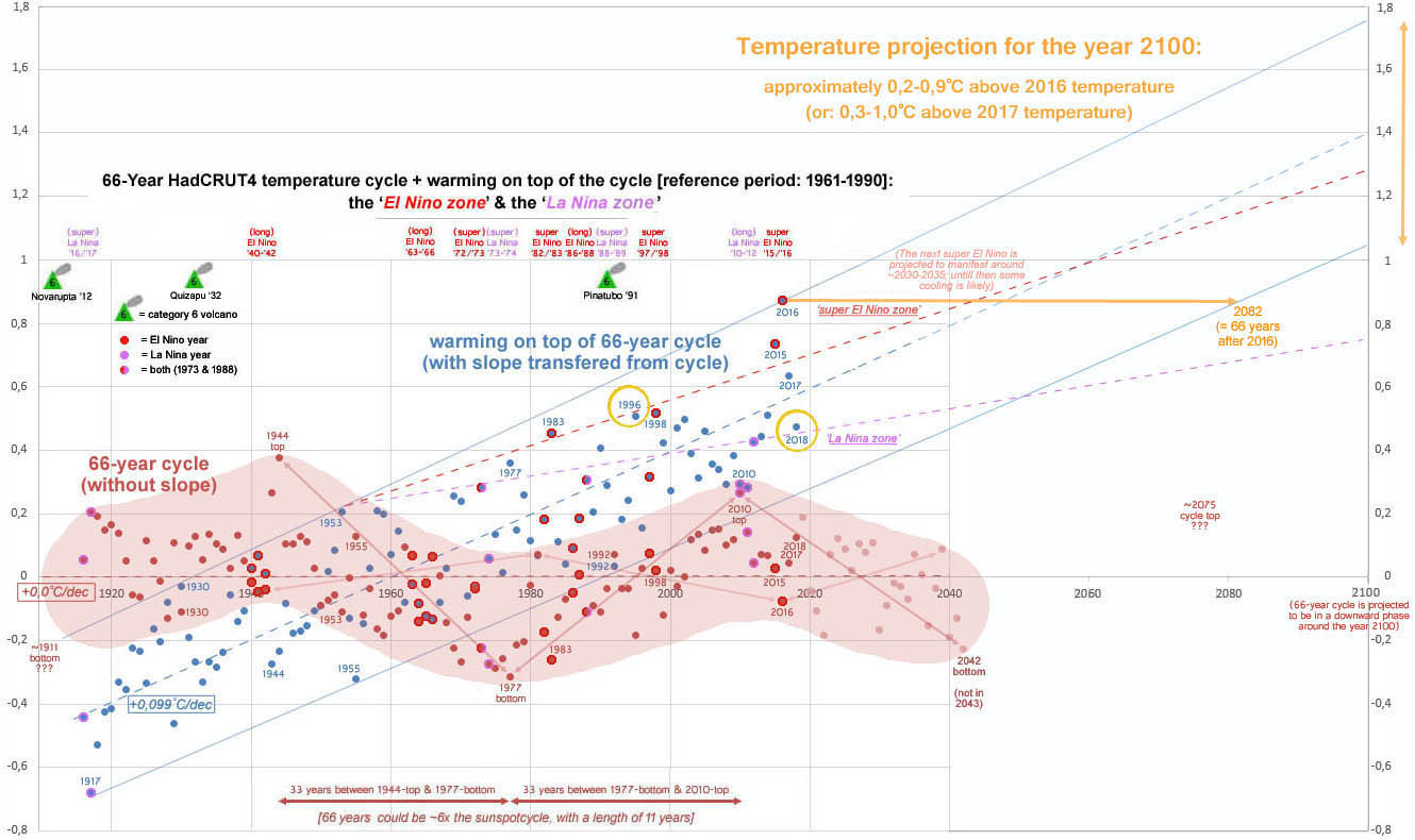
Figure 3: The corrected 66-year cycle (oscillation without slope) +
the corrected warm-up on top of the cycle (with slope); both are derived from the HadCRUT4 temperature series.
Additional quantitative analysis (1916-2018): warming on cycle slope = +0,088°C p/d; cycle slope = -0,006°C p/d.
The perspective of figure 3 shows that in the current decade the years 2015, 2016 and 2017 are at the top side of the bandwidth of the corrected warming on top of the cycle; 2018 and all other years of the 2010s are at the bottom side of the trend channel.
In figure 4 the values of figure 3 have been transformed to the 5-year average based on periods that relate to half of an entire decade; the 2nd half of the 2010s has been calculated over the period 2015-2018 (the year 2019 is not taken into account).
The green arrows represent the warming on top of the 66 year cycle; the development of the green arrows shows that global warming on top of the cycle in the period 1995-2014 was close to zero. Figure 3 suggests that the so-called 'hiatus' (= a pause in the warming-up) already starts in the year 1996, it continued until 2014, and subsequently in 2018 the temperature returns to the temperature zone of the 'hiatus'. This shows that a larger 'hiatus' appears to be hidden inside the HadCRUT4 temperature series than what the HadCRUT4 series itself suggests. This implies that the pause in the warming-up appears to be masked by the 66-year cycle.
In de decade analysis of june 2019 it was determined that on the basis of a 70-year cycle, the warming since the 1970s has been overestimated by more than 49%. For a 66-year cycle, this percentage drops to just above 44% in the perspective of a decade of analysis; however, based on the method described in section VI, this percentage amounts to just above 47% (after removal of the ENSO cycle). This comparison indicates that the result based on the 66-year cycle is therefore slightly lower than the previously described result based on a multidecadal cycle with a duration of 7 decades.
Figure 4: HadCRUT4 5-year average (red/light blue), plus starting from the 1920s:
the 66-year cycle (purple) and the warming on top of the cycle (green).
The average for every decade is represented by the broad light-red columns & broad light-blue columns.
As a final remark, figure 4 shows that the previous remark with regard to the midpoint value in figure 2 also applies to figure 4. A correction for this would result in a decrease of all values by -0.03°C; for the warming up on top of the cycle; however, this would not affect the outcome of an estimate involving the size of the structural overestimate resulting from to the 66-year cycle.
ADDITION: Due to the erratic course of the 66-year cycle described, the impact often fluctuates greatly when the analysis period is postponed, extended or shortened by for example 1 year. Therefore, in the perspective of the definition of 'climate change' (which is defined according the classical definition in terms of changes in the average for a period of at least 30 years) little value can be attached to comparisons between 2 individual years. In anticipation to an analysis based on the 30-year average in section VII, an exception is made here just once for the sake of completeness with the following observations:
Based on the corrected warming on top of the cycle in figure 3 (see blue graph), it can be determined that the warming on top of the cycle for the year 2018 is only +0.05°C relative to the year 1999; this warming is relatively small compared to the +0.29°C temperature difference between those years in the HadCRUT4 series. This implies that in the perspective of figure 3 the overestimation due to the 66-year cycle amounts to more than 82% in a comparison between the years 1999 and 2018. Section VI describes two other perspectives where percentages are presented on the basis of a comparison between the years 1999 and 2018. In the perspective of Figure 12 (where the warming on top of the cycle has been recalculated after first removing the values of the ENSO cycle and then the 66 year cycle is removed) a temperature difference is found again of +0.05°C, which again results in the percentage just mentioned. However, in the perspective of Figure 13 (where first the ENSO cycle has been removed and then a conceptual sinusoid 66-year cycle is removed) a temperature difference of + 0.20°C is found, resulting in in an overestimation of just over 31%. This shows that temperature differences found between individual years after removing de 66-year cycle, highly dependent on the format in which the 66-year cycle is represented. In general, a comparison between individual years might become more realistic in the perspective of figure 13; although here as well, account must still be taken of the possibility that all kinds of natural fluctuations (under the influence of for example: the sunspot cycle or category-6 volcanism) can potentially cause large differences in comparisons between successive years. Climate primarily is defined in terms of changes in the average over a period of at least 30 years; comparisons over a shorter period of time ought to be avoided by principle, unless for example the average over a period of 30 years is used in a comparison between the two individual years. For this reason no value can be attributed to the percentages just mentioned.
III - Projection for the year 2100: 0.2-0.9°C warming on top of record year 2016
The rising trend channel in figure 3 indicates that the warming on top of the corrected 66-year cycle for the remainder of the 21st century up to the year 2100 may be in the order of 0.2-0.9°C relative to the record year 2016. This projection overlaps the bandwidths of the three basic scenarios that the United Nations International Climate Panel (IPCC) outlines in its report of October 2018; figure 5 shows that the projection in the first half of the 21st century is found in the lower half of all three CO2 reduction scenarios of the IPCC.
The IPCC graph shows a projection based on the year 2017. Because the year 2017 is at a relatively high point in the trend channel for the warming on top of the 66-year cycle, this explains why the interrupted green line ends at a relatively high point of the described bandwidth of 0.2-0.9°C.
![Figure 5: Adjusted graph from the IPCC oktober 2018 report [page 8]</a> + a projection derived from the (corrected) 66-year cycle.](http://klimaatcyclus.nl/klimaat/pics/IPCC-temperature-projections-for-the-year-2100.jpg)
Figure 5: Adjusted graph from the IPCC oktober 2018 report [page 8] + a projection derived from the (corrected) 66-year cycle.
All three IPCC scenarios show a small temperature decrease in the 2nd half of the 21st century based on achieving a decrease in CO2 emissions from 2020 + a decrease to zero within a few decades.
The IPCC chart shows a gray line that represents a compilation of the monthly data of 4 temperature datasets: the HadCRUT4, the GISSTEMP, the Cowtan-Way & the NOAA dataset. The IPCC graph also shows a solid orange straight curve that is being described by the IPCC to represent an "estimate" derived from the gray line. The broken orange line represents the IPCC projection for the first half of the 21st century; it's slope is indicative for an expected temperature rise of around 0.20°C per decade.
A comparison between the interrupted orange line of the IPCC and the interrupted green line based on the corrected trend channel described in the previous paragraph, indicates that the IPCC most likely did not take into account the effect of natural variability due to the upward phase of the 66 year cycle. The rising momentum at the beginning of the IPPC's solid orange line can be understood to represent the direct result of the transition from the downward phase of the 66-year cycle to it's upward phase - the turning point was reached in the year 1976. The 'acceleration' in the upward movement of the orange curve between 1960 and 1980 can be recognized to represent a direct result of the natural variability resulting from the 66-year cycle.
Next to the warming trend of 0,099°C per decade, the oscillating movement of the 66-year cycle may also be taken into account; in figure 5 this is shown as a continuous wavy green line that ends in the year 2100. In this perspective, the multidecadal cycle is expected to be in it's lower phase around the year 2100; as a result of this the net warming compared to the year 2016 could remain limited. Also, because the slope of the downward phase of the cycle is even slightly steeper than the slope of the warming on top of the cycle (figure 12 in paragraph VI shows that this phenomenon is also present after removal of the ENSO cycle), the projected warming could turn out to be limited at the end of the 21st century. If the described trend channel persists, account may be taken to expect temperatures that are logically more likely closer to the center or the bottom of the bandwidth than to the top; a warming scenario that remains close to zero compared to the temperatures in the current decade is not necessarily unlikely.
The complexity of the climate system causes all kinds of temperature fluctuations that result from natural variability. A kind of irregular sawtooth movement is a typical phenomenon that can become manifest in a large number of perspectives, such as: daily-, weekly-, monthly- and annual fluctuations. Sawtooth movements are also found at the perspective of several years, decades, centuries and even millennia.
The Dutch KNMI acknowledged early in 2019 that natural variability is understood only moderate ("matig")13; therefore one should take into account the possibility that various natural oscillations are involved - the ENSO cycle has most likely the largest impact in the perspective of the annual variations. In section VI figure 13 shows a profound picture of the influence of the 3 most important cycles: the ENSO cycle, the sunspot cycle and the 66-year cycle. Figure 13 also shows a projection for the year 2100 with e.g. the influence of volcanism taken into account; it also exhibits the projection that the IPCC uses for the first half of the 21st century.
IV - Annual growth CO2 correlates highly with ENSO cycle
In November 2018 the Dutch KNMI published an update about the development of global warming and the increase in CO2 in the year 20184. The following passage + the attached graph (see figure 6) from the update raises question about the exact impact of the El Ninos on global warming over the years since 1940:
"De temperatuur in 2018 wordt ongeveer 0,84 graden hoger dan het gemiddelde over 1951-1980, zo'n 1,1 graad warmer dan 1880-1900. Dit ligt ongeveer op de paarse trendlijn: dit is wat we nu ongeveer verwachten op basis van de hoeveelheid CO2 in de lucht. Alleen de jaren 2015, 2016 en 2017 waren warmer. Dit kwam in 2015 en 2016 grotendeels door een sterke El Nino, die de wereldgemiddelde temperatuur even boven de trendlijn optilt. Dit was ook in 1997/98 het geval, en verder terug bijvoorbeeld in 1940/41. Grote vulkaanuitbarstingen, zoals die van Pinatubo in de Filipijnen in 1991, koelen de aarde de twee jaar er na juist af doordat ze zwavel in de stratosfeer brengen. De invloed van de zon is klein."
[The temperature in 2018 will be approximately 0.84 degrees higher than the average for 1951-1980, and about 1.1 degrees warmer than 1880-1900. This is roughly on the purple trend line: this is approximately what we now expect based on the amount of CO2 in the air. Only the years 2015, 2016 and 2017 were warmer. This was largely due to a strong El Nino in 2015 and 2016, which raises the world average temperature just above the trend line. This was also the case in 1997/98, and further back, for example, in 1940/41. Large volcanic eruptions, such as that of Pinatubo in the Philippines in 1991, cool the earth down in the subsequent two years by bringing sulfur into the stratosphere. The influence of the sun is small.]
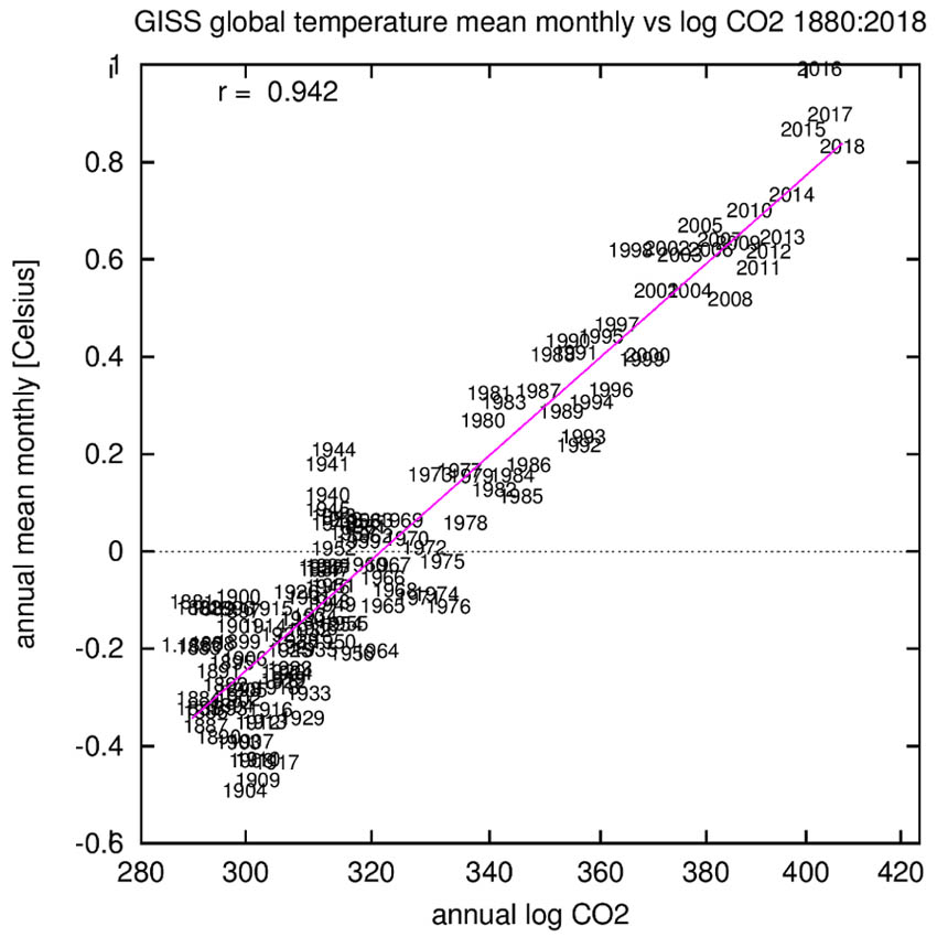
Figure 6: the correlation between CO2 & GISS temperature [1880-2018] is +0.942 (KNMI)4.
According the HadCRUT4 series, the worldwide temperature difference between the period 1951-1980 (with an average of -0.056°C) and the year 2018 (with an average of 0.597°C) was only + 0.653°C. This increase is more than 0.18°C lower than the KNMI description based on the GISS temperature series, which implies that the description of the KNMI based on the GISS temperature series is more than 28% higher than the HadCRUT4 series.
In section II was explained why comparisons based on the annual average of individual years should generally be discouraged. The same can actually be said with regard to correlations, because a correlation gives no information about cause and effect. However, correlations based on a period of at least 30 years do offer an interesting and also valid perspective to be taken into consideration.
Figure 6 shows a graph featured with the correlation between CO2 & the GISS temperature series which is quite high for the period 1880-2018: r = 0.942. Possibly the KNMI might have estimated the warming based on the GISS temperature series a bit too high; however, the correlation between HadCRUT4 and CO2 does yield a likewise high result for the period 1880-2018, namely: r = 0.92 (p = 0.000) - see Figure 7A. The same result is also found for the period from the mid-20th century 1951-2018: r = 0.92 (p = 0.000) - see figure 7B.
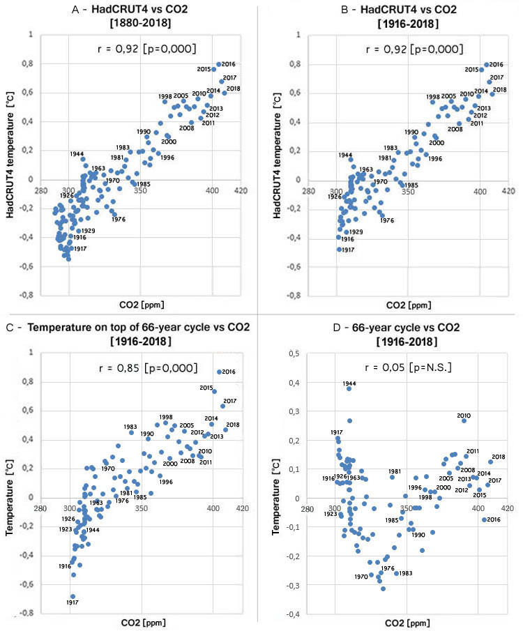
Figure 7: Correlation between CO2 with: (A) HadCRUT4 temperature 1880-2018, (B) HadCRUT4 temperature 1916-2018, (C) heating on top of corrected 66-year cycle 1916-2018, (D) corrected 66-year cycle 1916-2018. The correlations were calculated using average CO2 values presented by the NOAA from the year 1959, and values presented by the 2 Degrees Institute for the period prior to 1959.
Figures 7C and 7D show the result for in respective: the (corrected) warming on top of the cycle and the (corrected) 66-year cycle.
In june 2019 was demonstrated that the multidecadal cycle can lead to a substantial overestimation of the structural impact of global warming; a similar issue also arises in the perspective of CO2:
'To what extent does the 66-year cycle play a role in the correlation between CO2 and temperature?'
An answer for this question can be found, for example, via a comparison between CO2 and the following three perspectives respectively: (1) the HadCRUT4 series [HadCRUT4], (2) the corrected warming on top of the 66-year cycle [warming on cycle], 3) the corrected 66-year cycle [cycle]. Below the correlations for these three perspectives are shown for 10 periods:
• Correlation CO2 in period 1851-2018: HadCRUT4 (r=+0,91; p=0,000); [data cycle not available for 1850-1915]
• Correlation CO2 in period 1878-2018: HadCRUT4 (r=+0,91; p=0,000); [data cycle not available for 1880-1915]
• Correlation CO2 in period 1886-2018: HadCRUT4 (r=+0,92; p=0,000); [data cycle not available for 1880-1915]
• Correlation CO2 in period 1916-2018: HadCRUT4 (r=+0,92; p=0,000); warming on cycle (r=+0,85; p=0,000); cycle (r=+0,05; p=N.S.)
• Correlation CO2 in period 1944-2018: HadCRUT4 (r=+0,91; p=0,000); warming on cycle (r=+0,82; p=0,000); cycle (r=+0,32; p=0,002)
• Correlation CO2 in period 1952-2018: HadCRUT4 (r=+0,92; p=0,000); warming on cycle (r=+0,79; p=0,000); cycle (r=+0,54; p=0,000)
• Correlation CO2 in period 1977-2018: HadCRUT4 (r=+0,92; p=0,000); warming on cycle (r=+0,68; p=0,000); cycle (r=+0,68; p=0,000)
• Correlation CO2 in period 1985-2018: HadCRUT4 (r=+0,89; p=0,000); warming on cycle (r=+0,69; p=0,000); cycle (r=+0,55; p=0,000)
• Correlation CO2 in period 1998-2018: HadCRUT4 (r=+0,70; p=0,000); warming on cycle (r=+0,47; p=0,016); cycle (r=+0,19; p=N.S.)
• Correlation CO2 in period 2000-2018: HadCRUT4 (r=+0,73; p=0,000); warming on cycle (r=+0,57; p=0,006); cycle (r=-0,03; p=N.S.)
ANALYSIS: All periods show a (very) significant correlation between CO2 and the HadCRUT4. It also appears that in the periods from 1916 the correlation is also (very) significant between CO2 and the warming on top of the cycle. The 66-year cycle does not form a significant correlation with CO2 in the 1916-2018 period; however, for various periods from 1944 it appears that the 66-year cycle did make a (very) significant contribution to the correlation between CO2 and the HadCRUT4. These last correlations form a clear indication (read: confirmation) that the cycle causes a complication when studying the relationship between CO2 and temperature.
The correlations involving the cycle can be explained easily: for both the 66-year period between 1952-2018 and the period 1977-2018, the cycle moves around the bottom in the first decades and it moves around the top in the last decades. This results in a significant positive correlation between CO2 and the cycle, which produces a significant contribution to the significant positive correlation of +0.92 between CO2 and the HadCRUT4 temperature series in the 1952-2018 period. By logics this effect is likely even greater in the period 1977-2018 (than in the period 1952-2018) because in 1978 the cycle reaches it's lowest point very early in this perspective, which subsequently results in a positive correlation between CO2 and the 66-year cycle.
In addition, the ratios between the numbers shown suggest that the impact of the cycle may increase as the period goes less far back in time. In the last 2 periods the cycle does not in itself add a significant weight; however, the last example for the period 2000-2018 shows that even a negative correlation between CO2 and the cycle appears to deliver net a contribution to the significance level of the correlation between CO2 and the HadCRUT4.
The analysis above shows clearly that the 66-year cycle causes a major complication. Both in the periods from the peak of the cycle (1944) and the bottom of the cycle (1977), as well as the periods that relative to the year 2018 represent 2 full oscillations (1878) and 1 full oscillation (1952), and the period from the last super El Nino in the 20th century (1998), as well as for the entire 21st century (2000), shows that the cycle has made consistently a contribution that in each of these examples results in some amount of overestimation regarding the correlation between CO2 and the HadCRUT4 temperature series.
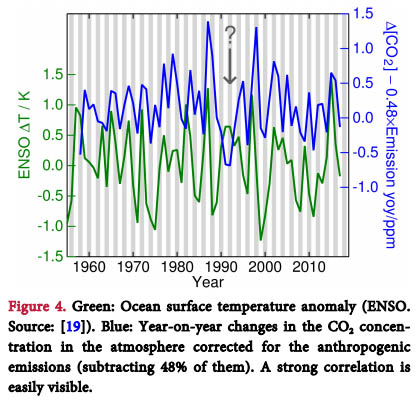
In the introduction was mentioned based on Henry's law, that the ENSO cycle also plays a significant role in this perspective; figure 8 shows that the ENSO cycle largely determines the annual growth of CO2 in the atmosphere.
Figure 8 [Figure 4]: The ENSO cycle correlates highly with the annual CO2 increase in the atmosphere; the Pinatubo volcanic eruption in 1991 may be held directly responsible for the only clear disturbance of the overall pattern, the effect is manifested in the graph in the year 19928. CO2 phasing is usually nearly 6 months behind ENSO cycle15 - this order is not surprising because this typical pattern (where CO2 lags temperature, not the other way around) is also found in: the day/night (diurnal) cycle, the seasonal cycle, and also in the ice age cycle (more details are described in the discussion, see section XII). By the way, the annual growth of CO2 also correlates high with precipitation - the same order is found here as well: CO2 follows the precipitation and not the other way around16. Voor meer details over de correlatie tussen de ENSO cyclus en de jaarlijkse groei van CO2, see: HERE and HERE.
An additional analysis is presented below for illustration on top of the relationship described in figure 8:
The EONI is used here with a delay of 6 months; attention has been drawn to the period from 1959 - the starting year of the first instrumental CO2 measurements on Mauna Loa (Hawaii). The correlation between the ENSO cycle and the annual growth of CO2 indeed is significant for both the period 1959-2018: r = 0.34 (p=0.004), the period 1959-1999: r = 0.41 (p=0.004) , as well as in the 21st century: r = 0.70 (p=0.000). The Pinatuba eruption in particular had a lowering effect on correlation in both 1991 and 1992; without these 2 years, the correlation for the remaining years in the period 1959-1999 rises to r = 0.48 (p=0.001).
When the period involving the 2nd part of the 20th century is split, it appears that the correlation between the ENSO cycle and annual CO2 growth has steadily increased, because in the period 1959-1979 it was not yet significant: r = 0.30 (p=N.S.); however, there was a significant relationship between 1980 and 1999: r = 0.48 (p=0.017). Subsequently, the correlation in the succeeding decades becomes steadily stronger in the 21st century; for the period 2000-2009 the correlation is: r = 0.72 (p=0.009) and for the period 2010-2018: r = 0.77 (p=0.008).
This pattern may evoke associations such as the question: "Has the growth of CO2 possibly caused a stronger ENSO cycle?". This question cannot be answered positive for the last 3 decades; when the years 1991 and 1992 are not taken into account (due to the impact of the Pinatubo eruption), this results for the remaining years 1990-1999 (ie without 1991 and 1992) even in the highest correlation (slightly higher than in the 2010s and 2000s respectively): r = 0.80 (p = 0.008). In short, the correlation has actually remained more or less stable over the past 3 decades when the impact of the 2 years around the Pinatubo eruption is not taken into account. Therefore there is no clear evidence for a cumulative effect of the increase in CO2 in the atmosphere on the ENSO cycle, since the correlation has remained stable. Meanwhile, in the period 1990-2018 atmospheric CO2 grew from 353ppm to 408ppm: a rise of more than 15%; also, according the NOAA the relative forcing of CO2 in these 29 years has increased by no less than 60%.
The next section V shows that both the 66-year cycle and the ENSO cycle have contributed, each with unique dynamics, in the formation of the complex relationship between CO2 and temperature. Among others an analysis is presented which demonstrates that in between super El Nino peak year periods, the correlation between the annual growth of CO2 with both HadCRUT4 and (corrected) warming on top of the 66-year cycle appears to have slowly weakened in the period since 1959.
V - 21st century: correlation temperature-CO2 based on 66-year cycle & super El Nino
Figure 9 concerns an illustration presented by the NOAA describing the annual growth of CO2. A striking characteristic in this graph shows that the average annual growth of CO2 in the 1980s was slightly higher compared to the 1990s. This is mainly due to the 2 strong El Nino periods that occurred in the 1980s; during that decade, the absorption of CO2 in the ocean system has been relatively low. This partly explains how the average annual growth of CO2 in the atmosphere in terms of the number of particles per million (ppm) in the 1980s became netto higher than in the 1990s.
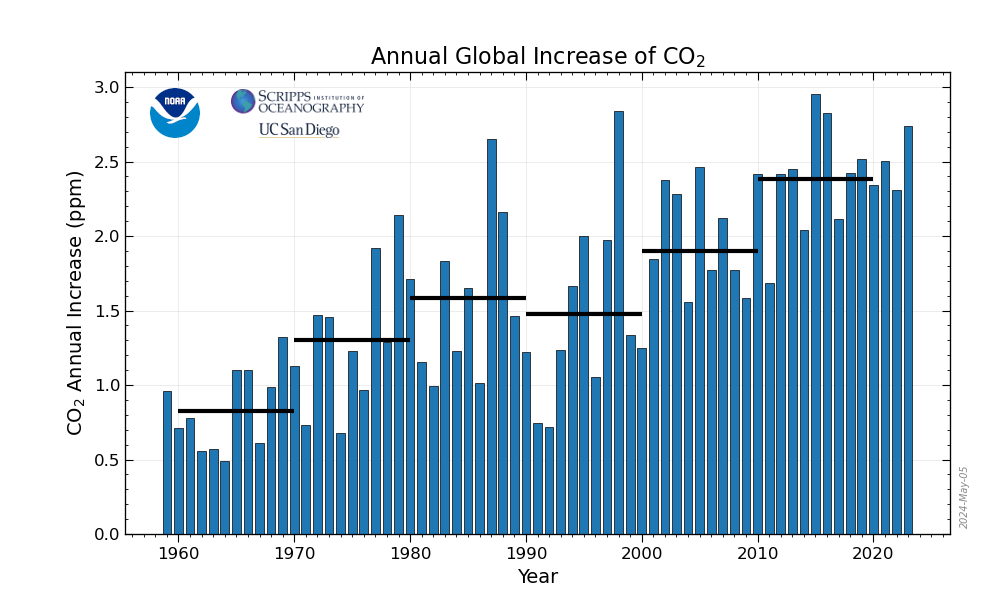
Figure 9: Annual growth of CO2 in the atmosphere.
The edited version of the NOAA graph in figure 10 shows that the greatest stagnation of growth in the early 1990s coincides with the Pinatubo volcanic eruption in June 1991. Also, the CO2 graph presented by the 2 Degrees Institute confirms: after the year 1991 and especially 1992 the CO2 level exhibits limited growth. The graph of the NOAA shows that the percentage of CO2 growth in 1992 even reached the lowest level since 1974.
This is a strong indication that 'mother nature' is able to play a significant role in the amount of annual growth of CO2 in the atmosphere. In addition to the influence of volcanism, the ENSO cycle is also a major determining factor for the growth of CO2 in the atmosphere every year7,8; this becomes also evident from the fact that the 4 highest peaks in the graph of the NOAA all concern El Nino years.
Figure 10: The correlation(s) between CO2 and HadCRUT4 temperature series; significant correlations are found only in some of the periods that overlap with the upward phase (1977-2010) of the 66-year cycle.
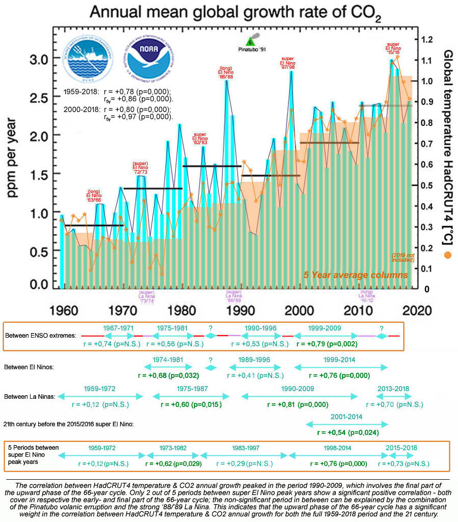
Figure 10 shows the HadCRUT4 temperature series combinated with the annual growth of CO2 in the atmosphere; the correlation is significant for both the entire 1959-2018 period (r = 0.78; p=0.000) and the period that relates to the 21st century: 2000-2018 (r = 0.80; p=0.000). The correlations based on the 5-year periods are slightly higher for both the entire period and in the 21st century. At the bottom of Figure 10, the correlations between the two factors are also shown for various periods between the ENSO extremes (read: the strongest El Nino and La Nina years, which are also shown in figures 1 to 4); periods with a duration of only 2 years are indicated with a '?' sign because no correlation can be calculated for a period of just two years.
Figure 10 shows e.g. that in various periods between ENSO extremes the correlation is not significant, but the values are all positive. Only 2 of the 5 periods between the super El Nino peak years show a significant correlation; these periods both relate to the start and end phase of the upward movement of the cycle. The highest value is found in the period 1990-2009, which corresponds to the last part of the upward movement of the 66-year cycle. The non-significant period in between (1983-1997) can be explained by the combination of the Pinatubo eruption (which is included in category 6 on the volcanic activity scale) and the strong '88 / '89 La Nina. The combination of these patterns suggests that the upward movement of the 66-year cycle (which relates to the period 1977-2010 - see also figures 2 to 4) plays a significant role in the development of the correlation between the HadCRUT4 and the annual growth of CO2 in the atmosphere.
Figure 11 shows the (corrected) warming on top of the 66-year cycle combined with the annual growth of CO2 in the atmosphere. For the entire 1959-2018 period, a slightly higher correlation was found in both the individual years and the 5-year periods compared to the correlation between HadCRUT4 and the annual CO2 growth (relative to figure 10). However, in this perspective the correlation for the years in the 21st century is clearly slightly lower than for the entire period; the value for the 5-year average has also fallen relative to the corresponding value in figure 10.
Figure 11: The correlation between CO2 and (corrected) warming on top of the 66-year cycle; rather remarkable is that the correlation for the individual years in the 21st century is lower than for the entire period.
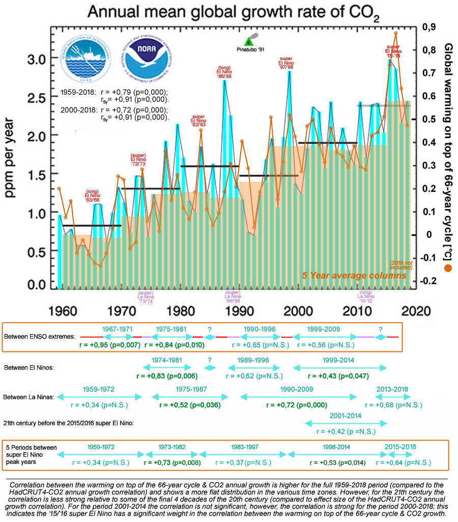
Figure 11 shows the correlation with the highest level of significance for the period 1990-2009. The periods with non-significant correlations that relate to at least part of the 21st century show, in particular from the period 1999-2009, that the '97 / '98 super El Nino probably made a major contribution to the emergence of the significant correlation for the period 1990-2009. Moreover, it is also noticeable that apart from the period 1990-2009, all four described periods that are entirely within the period of 1967-1982 produce the other highest correlations. For example, three of the four periods that are entirely related to the 21st century show a non-significant correlation (only the correlation for the entire 21st century is significant). In short, this pattern shows a clear difference with the perspective of figure 10 where the weight of the correlations is much more spread over the period that starts after the '72/'73 (super) El Nino.
It is also striking that a clear trend is observed in the four periods found in the perspective of the 'ENSO extremes' (see the upper frame at the bottom of figure 11); the power of the correlation has declined constantly in time. This suggests that the extremes of the ENSO cycle play a significant role in the development of the correlation between the warming on top of the 66-year cycle and the annual growth of CO2 in the atmosphere. As only El Ninos cause warming up in the atmosphere (this does not apply to La Ninas), it becomes obvious that the super El Ninos may play a key role in this.
A striking picture is found in the listing below involving the periods between the super El Nino peak years. The correlation is significant in 3 of the 5 periods between the super El Nino peak years; however, in 2 of these 3 periods there is only a relatively weak correlation. Moreover, in 2 of the 5 periods there is a clear negative correlation value - even though both negative values are non-significant.
Correlation HadCRUT4 vs CO2 (+ the correlations in the 5 periods between super El Nino peak years):
• 1959-2018: r = +0,93 (p=0,000)
• 1959-1972: r = -0,31 (p=N.S.)
• 1973-1982: r = +0,61 (p=0,029)
• 1983-1997: r = +0,67 (p=0,003)
• 1998-2014: r = +0,45 (p=0,036)
• 2015-2018: r = -0,83 (p=N.S.)
Correlation warming on top of 66-jarige cyclus vs CO2 (+ the correlations in the 5 periods between super El Nino peak years):
• 1959-2018: r = +0,79 (p=0,000)
• 1959-1972: r = +0,00 (p=N.S.)
• 1973-1982: r = -0,05 (p=N.S.)
• 1983-1997: r = +0,21 (p=N.S.)
• 1998-2014: r = -0,12 (p=N.S.)
• 2015-2018: r = -0,71 (p=N.S.)
Rather remarkable is that in the perspective of warming on top of the 66-year cycle vs CO2 no significant correlation was found in none of the five periods between the super El Nino peak years. Moreover, a positive value is found in just only one of these periods. Although this pattern in the results is not significant, it gives the impression that the positive correlation between CO2 and global warming on top of the cycle may have been largely caused by the ratio in the surplus of 4 super El Nino peak years versus only 2 super La Nina peak years. These La Nina peak years each shower a lower level of intensity compared with the last 3 super El Nino peak years.
From figure 10 and figure 11 combined one can derive that both in the entire 1959-2018 period and in the perspective of the 21st century, the significant correlation between CO2 and HadCRUT4 apparently originates from the combination of the upward movement of the 66-year cycle and the super El Nino peak years.
Actually, after correction for the ENSO cycle, there is a warming of + 0.664°C in the period 1959-2018, while the temperature increase in this period according to the HadCRUT4 is + 0.580°C. This could very well induce the impression that the ENSO cycle has masked part of the warming up during this period; however, if the impact of the 66-year cycle is also taken into account, this effect disappears. For, in the next section the warming after first removing the ENSO cycle and then the 66-year cycle is calculated in 2 different ways. The result for the period 1959-2018 yields a residual warming of + 0.528°C (based on the empirical data) and + 0.596°C (based on a conceptual cycle); both values relate to the past 59 years and result in a warming-up rate of, in respective: + 0.089°C per decade and + 0.101°C per decade - which is approximately half of the projection that the IPCC uses for the coming decades (see figure 5 and figure 13).
A more advanced step is made in the next sections, which describe the impact of both cycles each and the impact of the two cycles combined. Section VI will also show that the speed of warming in recent decades in particular has been overestimated due to the 66-year cycle. Subsequently, section VII will show that the alleged 'acceleration' in global warming since the 1970s can almost entirely be attributed to the 66-year cycle. It is demonstrated that both the structural impact of the temperature rise and the causal relationship between the rise in temperature and the 'acceleration' in the rise of CO2 in terms of the number of ppm, are overestimated due to the 66-year cycle.
VI - 21st century: warming rate 69% lower after removal of 66-year cycle & El Nino
The June 2019 article raised the question whether the definition of climate in terms of the "average over 30 years" is appropriate to prevent natural variability (involving the multidecadal cycle) from being regarded as climate change. This section examines the impact of the 66-year cycle and the ENSO cycle combined based on the average temperature rise over 30 years found in individual years. However, first an analysis is made based on the (corrected) 66-year cycle in combination with the ENSO cycle, and then a control analysis based on a conceptual sinusoidal cycle of 66 years in combination with the ENSO cycle.
Estimates made by El Nino experts for the contribution of the '15/'16 super El Nino to the temperature cover a bandwidth that varies from 0.07-0.2°C; the top side of this bandwidth is being used by employees of the agency behind the British HadCRUT4 temperature series.
A calculation for the relative impact of the ENSO cycle in the perspective of global warming in the 21st century up till 2016, requires the value of the ENSO cycle in both the year 1999 and 2016 to be taken into account.
Based on the Ensemble Ocean Nino Index, an exact estimate can be made for the contribution of the ENSO cycle for individual years. Assuming a delay of 6 months (a representative period for the climate system to manifest the impact of the ENSO cycle around the world), the contribution of the super El Nino in 2016 can be +0.169°C estimated (= 10% of the average EONI value for the period July 2015 uptil including June 2016). This value is slightly higher than the estimate of the NASA5, but well within the bandwidth of 0.07-0.20°C based on the estimates of El Nino experts. However, in the year 1999 the ENSO cycle produced a negative EONI value: -0.117°C (= 10% of the average EONI value in the period July 1998 through June 1999).
This means that the ENSO cycle made a positive contribution to global warming in 2016, but in 1999 the ENSO cycle made a negative contribution. Therefore the ENSO cycle caused a net temperature difference of +0.286°C between the years 1999 and 2016, which represents no less than 58.2% of the 0.401°C temperature difference between the two years, based on instrumental measurements according to the HadCRUT4 temperature series. However, it has been stated in section II that little value should be putten to comparisons between individual years.
A complication for a calculation of the impact of the ENSO cycle & the 66-year cycle combined involves the fact that by principle both cycles influence each other. Therefore, when studying the impact of both cycles together, it is desirable to calculate the impact of the 66-year cycle after the ENSO cycle has been removed from the HadCRUT4 temperature series. The result for the 66-year cycle after removal of the ENSO cycle is referred to as the 'bare 66-year cycle' and is shown in Figure 12. Based on the tops and the bottoms plus the width of the cycle channel, is determined that the bare 66-year cycle in this perspective (without the influence of the ENSO cycle) has an amplitude size of 0.12°C (amplitude size of the ENSO cycle is around 0.20°C). Moreover, the cycle appears to have a more regular course in this perspective than the cycle shown in figures 2 and 3.
Figure 12: bare 66-year cycle + warming on top of cycle after removal of the ENSO cycle.
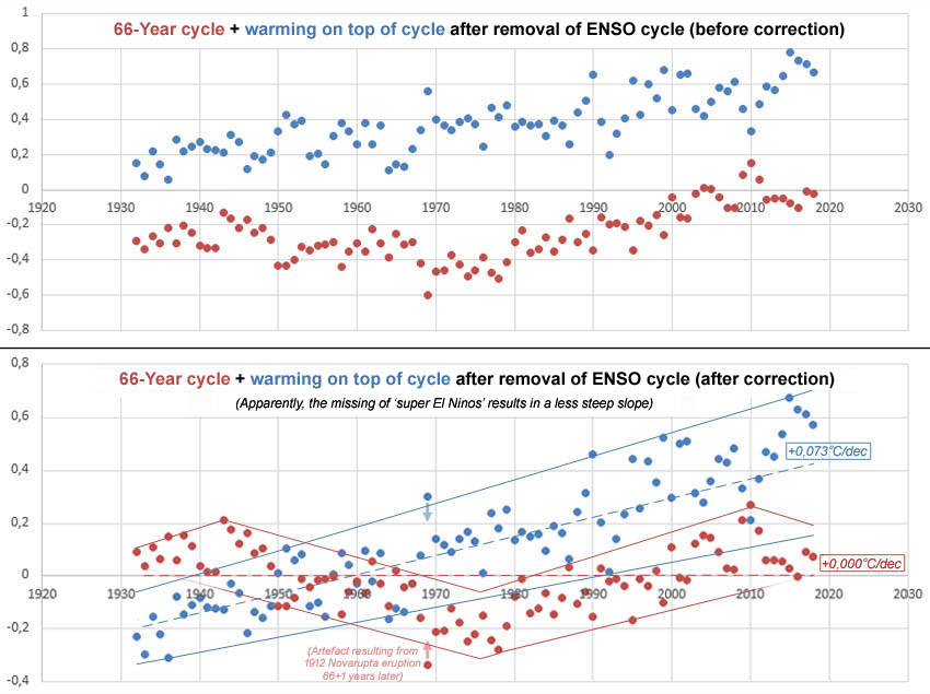
NOTE: In figure 12 the values for the year 1969 are not taken into account because they concern an artifact resulting form the Santa Maria volcanic eruption in the year 1902; in the bare 66-year cycle the impact involved yields a relatively low value for the year 1969 (+ a side effect by means of relatively high value the for warming on top of the 66 year cycle).
Additional quantitative analysis (1932-2018): warming on cycle slope = +0,086°C p/d; cycle slope = -0,000°C p/d.
Subsequently, based on the 'bare 66-year cycle' with an amplitude of 0.12°C as shown in figure 12 (which is found after removal of the ENSO cycle), a total perspective has been developed in which the 'bare 66-year cycle' is replaced by a 'conceptual 66-year cycle' with a sinusoid shape (the same correction described in section II has been applied in the calculation process); the result is shown in figure 13.
(Click HERE fore the high resolution version of figure 13)
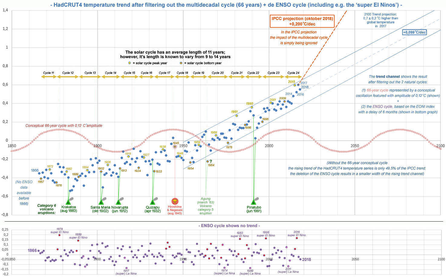
Figure 13: Warming on top of a conceptual 66-year cycle with an amplitude of 0.12°C (see the oscillating sine wave) after removal of the ENSO cycle; the ENSO cycle is shown in the lower part of the illustration. The most important volcanic influences are also featured + the influence of the sunspot cycle is made visible as well inside the upwardly directed trend channel.
Additional quantitative analysis (1950-2018): warming on cycle slope = +0,101°C p/d; cycle slope = 0,000°C p/d.
There are now 2 perspectives available to make a comparison; on the one hand, the rate of warming on top of the HadCRUT4 and, on the other, the warming that remains after removal of both the ENSO cycle and the 66-year cycle, respectively.
Subsequently, for each year separately for both the HadCRUT4 and for the warming in both perspectives (after removal of the ENSO cycle and 66-year cycle), the speed of the average temperature rise per decade has been calculated on the basis of the temperature difference compared to 30 years earlier. Just as an illustration for this approach, a calculation example is first presented based on the temperature difference compared to 30 years earlier, from which a first impression is distilled with regard to the impact of the combination of the 66-year cycle and the ENSO cycle on the HadCRUT4. In the following section, the last step is then taken on the basis of the 30-year average - in accordance with the fact that the 30-year average is also used in the traditional definition of 'climate change'.
TWO CALCULATION EXAMPLES: for the year 2018, an average temperature rise of +0.133°C per decade is found in the HadCRUT4 temperature series compared to 30 years earlier. In the perspective of the bare and conceptual cycle respectively, an average temperature rise of +0.117°C and +0.114°C per decade is found for the warming on top of the cycle involved. This calculation has been performed for all years of the current decade (2010s with the exception of 2019), all years of the 1990s and all years of the 1970s.
Calculation example 1: A comparison between the 1990s and the 2010s produces a rise in temperature in the HadCRUT4 perspective, where the average speed between the two periods has increased from +0.1010°C per decade in the 1990s to +0.169°C per decade in the 2010s. This results in a net increase in the speed of the temperature increase of +0.059°C per decade. However, in the perspective of the bare and conceptual cycle, the result of warming up on top of the relevant cycle is considerably lower, respectively: +0.017°C per decade and +0.019°C per decade. In short, after both cycles have been removed, the speed of the temperature rise is considerably lower in both perspectives compared to the HadCRUT4 temperature series. According logics the 66-year cycle likely had an inflationary impact on the temperature rise in the HadCRUT4 series. Based on the average of the perspective of the bare and conceptual cycle, the conclusion can be derived that from the calculated increase in the rate of HadCRUT4 temperature rise in the 21st century (based on a comparison between the years 2010s and 1990s) of +0.059°C per decade, just +0.018°C per decade can be labelled as the part that is not associated with the influence of the multidecadal cycle or the ENSO cycle. Therefore one can speak of an overestimation of the increase in the rate of temperature rise of no less than 227%; or it can be concluded that more than 69% of the increase in the rate of the observed temperature rise in the HadCRUT4 series is due to the impact of the combination of the 66-year cycle and the ENSO cycle.
Calculation example 2: On the basis of the same comparison between the 1970s and the 2010s, slightly higher percentages are found. In the perspective of the HadCRUT4, a temperature rise is found whereby the average speed between the two periods has increased from -0.024°C per decade in the 1970s (the negative value is due to the transition from the downward phase to the upward phase of the cycle) to +0.169°C per decade in the 2010s. This results in a fastening in the speed of the temperature increase of +0.193°C per decade. From the perspective of the bare and conceptual cycle, the result is considerably lower, respectively: +0.029°C per decade and +0.041°C per decade. In short, after removal of the two cycles in both perspectives the speed of the temperature rise is considerably lower compared to the HadCRUT4 temperature series. Logically, the multidecadal cycle in particular likely has an inflationary effect on the HadCRUT4 temperature rise. Based on the average of the perspective of the bare and conceptual cycle, the conclusion can be derived that from the calculated increase in the rate of HadCRUT4 temperature rise in the 21st century (based on a comparison between the years 2010s and 1970s) of +0.193°C per decade just +0.035°C per decade can be described as a part that cannot be associated to result from the influence of the multidecadal cycle or the ENSO cycle. One can speak of an overestimation of the increase in the rate of temperature rise of no less than 451%; or it can be concluded that over 81% of the increase in the rate of the observed temperature rise in the HadCRUT4 series is due to the impact of the combination of the 66-year cycle and the ENSO cycle.
The overestimation of the speed is therefore slightly greater in the comparison between the current decade and the 1970s than in a comparison with the 1990s. This is by no means surprising since in the 1970s the downward phase of the 66-year cycle changed to the upward phase, therefore the overestimation of the increase in the rate of temperature rise associated with that period is expected according logics to be larger. After all, at the beginning of the 1970s the HadCRUT4 temperature series was still decreasing due to the downward phase of the cycle; however, when the cycle is filtered out a more clear view is found on the underlying development without the influence of natural variability (in the form of the 66-year cycle and the ENSO cycle). Also, the size of this effect was taken in consideration in the initial approach where only the bare 66-year cycle (without removal of the ENSO cycle) was filtered out. Even in that case the effect appears to be greater in the 70s than in the 90s. For that initial approach the difference is considerably smaller between the two periods, but the average effect of both periods remains almost exactly the same compared with the perspective in which the combination of both cycles is filtered out in the perspective of the bare 66-year cycle.
From the calculation examples above can be deduced that the alleged 'acceleration' in the temperature rise (which is often attributed to CO2) is probably to a large extent the direct result of the combination of the following two causes:
Cause 1: The use of a too short period to calculate the average rise in temperature; after all, on the basis of a period of just 30 years, the 66-year cycle is currently causing an inflationary effect because the cycle has been in the high phase during the last two decades.
Cause 2: Underestimation of the influence of natural cycles on the speed of temperature rise; there is still a lot of incomprehension in the scientific literature and there is even denial of the 'hiatus' (the pause in the temperature rise) that has not only become visible in most global temperature series, for, since the super El Nino of the year 1998 it has also become visible in models for ocean heat content17 and surface temperature of large lakes worldwide18.
Unfortunately, mathematically, no estimate can be made here of the impact of the combination of the 66-year cycle and the ENSO cycle since the start of the industrial revolution; because the values for the ENSO values are available from 1866; the consequence from this is that the 66-year cycle values after filtering out the ENSO cycle are available from 1932. However, because the weight of the impact of both cycles gradually decreases for periods longer than 66 years, and in both cases it concerns a period that is longer than 1 full oscillation of the 66-year cycle, this impact could be estimated as zero for the period prior to the year 1932.
VII - 30-year average: acceleration in warming almost fully explained by 66-year cycle
In accordance with the definition of climate, is based on the 30-year average in figure 14 an impression is given for the development at: the HadCRUT4 temperature series (blue), the HadCRUT4 without the corrected 66-year cycle (red), and the two variants where the ENSO cycle has also been removed (green and purple).
The percentages show that the 30-year average of the HadCRUT4 has risen considerably more rapidly in the last 3 decades than in the 1970s and 1980s; however, the acceleration observed appears to be largely explained by the 66-year cycle - because only the HadCRUT4 graph shows an irregular course in the speed at which the temperature rises.
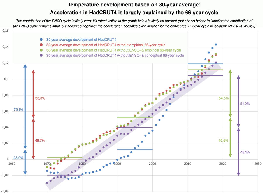
Figure 14: Acceleration in the 30-year HadCRUT4 average is largely caused by a 66-year cycle.
In Figure 14, the slope of the course within every decade also indicates the speed at which the 30-year average is rising. In the track of the series in which the ENSO cycle & the conceptual 66-year cycle is filtered away (purple), a number of things are striking:
• The trend channel shown (light purple) is remarkably narrow.
• A gradient is found in all five decades which at least partly corresponds with the slope of the light-purple trend channel.
• 2x a short period with an almost flat slope is found; this concerns the periods '73 -'75 and '91 -'93 that are separated by 18 years. It is also striking that a less sharp increase is found in the years 2009-2011 than in all other periods of 3 years in the graph. Figure 13 shows that for all three periods of 3 years the following applies: the first year is just in the upper half of the trend channel, after which the next 2 years are in the lower half of the trend channel. The first two of these 3-year periods take place on the way to a decline in the solar cycle and the third period takes place from a fall in the solar cycle.
The last phenomenon that relates to the three 3-year periods is only found in at most 2 of the 3 periods in the other three series. The other 3 series of years may not seem sufficiently sensitive to consistently detect this 'signal' within the solar cycle. This indicates that the sunspot cycle has a clear impact on the course of the 30-year average - this means that for a deeper study of the trend channel it is desirable to also remove the sun cycle.
In earlier sections, three different perspectives (see figure 3, figure 12 and figure 13) describe a trend channel based on the extreme values in the bandwidth using a visual analysis. For each perspective is based on the 30-year average a value was calculated for the speed of the temperature rise in the past 5 decades, i.e. on the basis of the years: 1970-2018. This means that, for example, the calculation for 1970 relates to the average value in the period 1941-1970).
Below is a summary overview of the values described in each figure based on the approach based on the extreme values, plus the values found on the basis of a calculated average value for the rate of the increase per decade (p/d):
• Figure 3: rise according extreme values: +0,099°C p/d; rise based on 30-year average: +0,089°C p/d
• Figure 12: rise according extreme values: +0,073°C p/d; rise based on 30-year average: +0,089°C p/d
• Figure 13: rise according extreme values: +0,099°C p/d; rise based on 30-year average: +0,101°C p/d
The average value of the 6 described speeds above listed is: +0.092°C per decade; based on the perspectives in which the ENSO cycle was first removed, the average is +0.090°C per decade. The result based on the 30-year average therefore appears at first sight to have yielded the most representative result in both analyzes based on the empirical data (= the corrected cycle based on figure 3 & bare cycle based on figure 12). This amounts to a trend rate of +0.09°C +/- 0.01 °C per decade, whereby for the year 2100 a downward correction of 0.1°C may be taken into account on the basis of an expected negative phase of the 66-year cycle. Subsequently, the randomness of the ENSO cycle also causes a potential deviation in the amount of a further 0.2°C.
The end result of this analysis for the year 2100 for the next 81 years results in an expected temperature increase of +0.65°C with a bandwidth that can vary from roughly +0.35°C to +0.95°C compared to the average temperature of the year 2017 (based on the average temperature of the year 2016, this forecast can be lowered by -0.1°C and based on the average temperature of the year 2018, the forecast can be increased by +0.1°C). This result corresponds fairly closely to the trend described in Figure 5, where a bandwidth was found compared to the year 2017 with a lower limit of +0.30°C and an upper limit of + 0.90°C. If it were found that the conceptual cycle should be used (based on a sinusoid with an amplitude of 0.12°C), then the numbers described for the year 2100 can be increased with a value of +0.1°C.
The average bandwidth of 0.35-0.95°C found above also falls neatly within the bandwidth described earlier in paragraph II in figure 4: 0.3-1.0°C (for the first perspective where the ENSO cycle has not been deleted).
The warming in the year 2100 could become limited to a lower value if, in the meantime, the ratio between El Nino events and La Nina events were to remain in balance, or would move towards more influence from La Ninas.
It can also be noted that in the perspective where after the removal of the ENSO cycle the empirical (bare) cycle has been used, the temperature peak that has arisen in addition to the 66-year cycle in recent years has already taken place in 2015; subsequently the value in 2016, 2017 and also in 2018 decreased every year. However, Figure 13 makes it clear that 2015 was a peak year in the solar cycle, so this remarkable effect might disappear in that perspective if the solar cycle were also filtered from the trend channel.
VIII - Four characteristics of the 66-year cycle
1 - A 66-year cycle was found with an amplitude of 0.12°C based on: half the average distance between the peaks & troughs, then after subtracting the width of the trend channel of the cycle (see figure 12).
2 - The natural variability inside the 66-year cycle has remained stable over a period of 70 to 90 years (see figure 13 and figure 12).
3 - The oscillation of the 66-year cycle can be simulated by means of a sinusoid with an amplitude of 0.12 °C (see figure 13).
4 - The 66-year cycle probably is around the year 2100 in it's lower phase (see figure 4 and figure 13).
IX - Five characteristics of the warming on top of the 66-year cycle
1 - Based on 3 perspectives, an average increase of +0.09°C per decade is found for the trend channel of warming on top of the 66-year cycle (the calculation is described in paragraph VII); in the perspective of a 66-year sinusoidal cycle, the increase is approximately +0.01°C higher - which results in an increase of +0.10°C per decade (see figure 13).
2 - No clear trend is spotted in the various perspectives that points towards a change in the amount of natural variability. Within the perspective of correcting only for the 66-year cycle, the variability within the warming on top of the cycle seems to have increased by around 16% in 1 century (in figure 3 this is reflected by a small divergence of the upward trend channel). After removal of the ENSO cycle, this natural variability appears to have doubled compared to the first perspective (see Figure 12). However, from the perspective of the conceptual cycle, the natural variability within the trend channel appears to have decreased slightly. These trends are fundamentally inconsistent, so no conclusions can be drawn from it.
3 - In the first perspective, all super El Nino years in the current decade are in the 'super El Nino zone'; all La Nina years are in the 'La Nina zone'; all other years proceeded between the 'super El Nino zone' and the 'La Nina zone' (see figure 3).
4 - Only in the two perspectives that include a removal of the ENSO cycle, the years 2015-2018 are at the top of the trend channel, those years also are found above all previous years. From 1990 (this is a peak year in the solar cycle in figure 13), the temperature in the period up to and including 2014 increased only slightly. The maximum increase compared to 1990 in this period, in both perspectives is no more than: just above +0.07°C (for the year 2015) & just above +0.06°C (for the years 2006, 2009 & 2011).
5 - Due to the Pinatubo volcanic eruption (category 6) in June 1991, the warming on top of the 66-year cycle reached the bottom of the upward trend channel in 1992 in the two perspective that include a removal of the ENSO cycle. This represents the lowest level reached since the 2nd half of the 70s.
In both perspectives a similar situation took place 28 years earlier in the year 1964 due to the Agung volcanic eruption (category 5); rather remarkable is that in the perspective of the empirical cycle also exactly 28 years earlier in the year 1936 was the last moment when the warming on top of the cycle arrived at the bottom level of the trend channel. Figure 13 shows that this happened 4 years after the Quizapu volcanic eruption (category 6) that took place in the year 1932 - notice: not shown in figure 13 is that in the meantime in the year 1933 also the Kharimkotan eruption (category 5) occurred. Incidentally, in 1991, in addition to the Pinatubo eruption, the Mount Hudson eruption (category 5) also took place. This means that the combination of 2 large volcanic eruptions took place within a period of one year only in the years '32/'33 and the year 1991.
The following is no more than a very speculative scenario: should a similar event occur again after 28 years, then a volcanic eruption would occur before October 2020 that might be sufficiently strong enough to make the warming on top of the cycle reach in 2021/2022 the bottom of the trend channel.
X - 66-year cycle may have a cosmic origin
In june 2019 it was described that the multidecadal cycle is mainly associated with the ocean system, whereby a relatively large weight is assigned to the 'Atlantic Multidecadal Oscillation' (AMO); however, the 'Pacific Decadal Oscillation' (PDO) and possibly also other ocean systems such as the 'Southern Oscillation' (SO) may also place some weight in the scale regarding the amplitude of the oscillation.
The multidecadal cycle is also related to solar activity via, among other things, the rotation speed of the earth. Figure 15 describes a theory in which the peak of the 66-year cycle is accompanied by a solar maximum in combination with a delay in the rotation speed of the earth; the low point of the 66-year cycle, on the other hand, is accompanied by a solar minimum with an acceleration of the earth's rotation speed19,20. This theory, incidentally, fits in seamlessly with another theory that describes that an acceleration of thermohaline circulation could possibly explain a significant part of the warming in the last decades of the 20th century21.
In the scientific literature, the 66-year cycle is also associated with the 11-year sunspot cycle based on six oscillations19,22,23.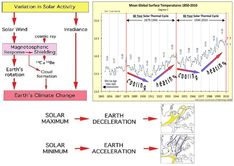
Figure 15: Solar activity & the 66-year thermal cycle described by N.A. Mörner (2010)19,20.
XI - Is the definition of 'climate' outdated?
The traditional definition of the climate suggests that natural fluctuations can be associated with the average temperature, humidity, air pressure, wind, cloud cover and precipitation over a period of at least 30 years24.
Since the 1990s, it has become clear that multidecadal oscillations are found in the ocean system that have some influence on global temperatures. In this article it is described that a 66-year cycle is found in the HadCRUT4 temperature series that is a controlling factor in the fluctuations in the average annual temperatures worldwide.
The logical consequence of this is that the "period of at least 30 years" in accordance with the traditional definition of climate according to the World Meteorological Association (WMO), should probably be extended to at least 66 years. A doubling to at least 60 years may also be sufficient. After all, only through an extension of the 30-year period mentioned in the definition, the impact of the multidecadal cycle (which is probably largely based on the combination of the cycles in both the Atlantic Ocean and the Pacific Ocean, possibly combined with the sunspot cycle) be neutralized. If this is not taken into account, the multidecadal cycle represents a major complication in determining climate change.
Researchers from the Dutch KNMI have established since at least 2012 that a 30-year period in the perspective of weather extremes is too short to separate climate change from the influence of natural variability:1,2
"... Generally such a climatological period is defined as a 30-years period, although we note that even 30 years may be too short to capture all natural climate variability"
It has become clear in this article that this point, in addition to the perspective of the weather extremes, probably also plays a crucial role in the perspective of the development of the average temperature worldwide. Because the impact of the natural variability associated with the 66-year cycle is insufficiently recognized; the result is that the impact of various climatic trends is currently overestimated due to the use of a climate definition that uses a far too short period of just 30 year.
Below is another illustrative example presented based on local research showing that the significance of this issue is possibly masked due to the "satellite age", when the most modern measurements have started at the end of the 1970s - only about 4 decades ago.
This spring (March 2019), a study on the Red Sea provided a description that explicitly stated that the impact of multidecadal cycles should also be taken into account for the mainland. Figure 16 concerns an illustration from this research involving the Red Sea; it presents a projection for the coming decades based on a cycle of "nearly 70 years" (which is associated with the AMO) after correction for the AMO. The following passage is a quote from the summary of this publication25:
"High warming rates reported recently appear to be a combined effect of global warming and a positive phase of natural SST oscillations. Over the next decades, the SST trend in the Red Sea purely related to global warming is expected to be counteracted by the cooling Atlantic Multidecadal Oscillation phase. Regardless of the current positive trends, projections incorporating long-term natural oscillations suggest a possible decreasing effect on SST in the near future."
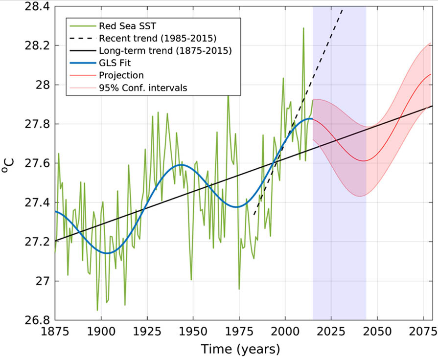
Figure 16: Red Sea projection of time series for sea surface temperature (SST) based on the superposition of linear trends and the low-frequency Atlantic Multidecadal Oscillation signal (red line), limited by the 95% confidence intervals (shaded red areas). The annual average SST is displayed in green. The continuous black line shows the trend based on the historical period (1880-2015); the black dotted line shows the trend based on the satellite era (1985-2015). The shaded blue area marks the period of the projected negative trends25.
In figure 16 it is described that the trend found in the 'satellite age' with regard to the temperature development of the Red Sea, yields a considerable overestimate compared to the AMO (the associated sinusoid oscillation has an amplitude of 0.16°C). An underlying long-term trend is found with an increase of only +0.043°C per decade, while under the influence of the AMO for the period 1980-2015 a trend of no less than +0.21°C per decade is found; this implicates an overestimation of the order of almost 400%.
The description presented by the researchers from Saudi Arabia shows a clear parallel with the description in this article for the HadCRUT4 in the perspective of global temperature development. The IPCC projection for the coming decades in the order of +0.20°C per decade as shown in figure 5 and figure 13 is a direct consequence of not recognizing the existence of the multidecadal climate cycle. Interestingly, in the 1990/1992 AR1 climate report the IPCC even predicted for the 21th century a temperature increase of +0.30°C per decade; in the perspective of this article this earlier even higher overestimation can be recognized to origin from the direct consequence of the fact that the highest momentum of the upward phase of the 66-year cycle was reached around the early 1990s.
XII - Discussion & conclusion
In summary, it has become clear in this article that the combination of the 66-year cycle + the ENSO cycle is responsible for more than 81% of the acceleration in warming based on the 30-year average since the 1970s, and more than 69% compared to the 1990s. A comparison between the 1970s, 1990s and 2010s shows that the assumed acceleration in global warming can almost entirely be attributed to the 66-year cycle. This also implies an overestimation due to the 66-year cycle regarding the structural impact for the correlation between temperature and CO2 in this period.
For the warming on top of the 66-year cycle a trend channel is found with a speed of +0.09°C per decade; this is about half the expectation communicated by the IPCC for the next few decades, namely: +0.20°C per decade. The observed trend is comparable to the result of +0.10°C per decade reported in a 2011 study based on the trend in sea surface temperature26. The observed trend results in a projection for the warming until the year 2100 (relative to 2017) with a bandwidth of +0.35°C to +0.95°C, including a corresponding midpoint of +0.65°C.
In the 20th century there was an imbalance in the ENSO cycle whereby more frequent and more intense strong El Nino periods occurred (relative to the strong La Nina periods); if nature restores this imbalance in the climate system in the 21st century through relatively more strong La Nina periods, the temperature prior to the year 2100 could possibly fall through the lower limit of the trend channel.
In the analysis of june 2019 is described that also for the temperature series GISS (used by NASA) and MLOST (used by NOAA) a similar oscillation pattern is found with peaks featured with 7 decades in between. The impact of the 66-year cycle is probably less strong in those two other series compared to the HadCRUT4. Based on the mutual differences between the series in the peak year 1944 and the off-peak year 1976, the following indicative estimates can be made (when a 66-year conceptual sinusoid cycle is used the values for the trend channels below become +0.01°C higher):
- 66-Year cycle in HadCRUT4 shows an amplitude of 0,12°C; trend channel: +0,090°C per decade.
- 66-Year cycle in MLOST shows an amplitude of ~0,100°C; trend channel: ~+0,108°C per decade.
- 66-Year cycle in GISS shows an amplitude of ~0,094°C; trend channel: ~+0,115°C per decade.
The values shown can be putten in perspective combined with two other natural cycles that have a much shorter oscillation but a larger amplitude, namely: the ENSO cycle (2-7 years; amplitude: ~0.2°C) and the sunspot cycle (9-14 years; amplitude: ~0,09°C). According to the current state of affairs in science, in the perspective of volcanism by principle one can not speak in terms of a cycle (nor an 'amplitude').
The method described above can be described as a form of a 'dissecting' of the temperature graph, with the ENSO cycle and the 66-year cycle removed from the HadCRUT4 temperature series. In other studies an attempt has been made to 'reconstruct' the temperature in the opposite direction; in such methods the ENSO cycle is removed first from the temperature graph. An example for this was recently described by K. Haustein et al. (august 2019), whose work was previously used in an analysis of Carbonbrief (december 2017). However, these models are based on (controversial) assumptions regarding the impact of aerosols (dust particles); in such reconstructions, the weight of greenhouse gasses is purposefully weighted on the basis of theoretical grounds through the assumption that aerosols provide considerable net cooling. This assumption is also always made in the climate models used by the IPCC. However, the uncertainty surrounding this assumption is so great that it can be stated at the same time that this assumption is insufficiently supported by both "both laboratory and field studies". It is therefore by no means surprising that the KNMI takes a neutral position with regard to the impact of 'aerosolen':
"Aerosolen spelen een belangrijke maar complexe rol in onze atmosfeer, in luchtvervuiling en klimaatverandering. Welke rol ze precies spelen in ons klimaat is nog onduidelijk."
[Aerosols play an important but complex role in our atmosphere, in air pollution and climate change. What role they play in our climate is still unclear.]
The current state of science is that it cannot be excluded that the role of the most important aerosol black carbon determines the net effect of aerosols in the form of heating. Aerosols can therefore be recognized as a speculative element in climate models. Aerosols belong to the core of the controversies in the climate debate the perspective of the scientific literature. Aerosols also play a role in the controversy in the climate debate about the nature and impact of changes in the cloud system.
In the IPCC report of October 2018 a projection is presented for the following decades in the first half of the 21st century; this projection corresponds to an expected increase of approximately +0.20°pC per decade (see figure 5 in section III).
Meanwhile, the IPCC alarm sounds. Since the early 1990s, some sources in the scientific literature make claims involving "unprecedented warming" in the 20th century in the context of the past 500 years27. Later, the Dutch KNMI also started talking about an 'acceleration' in the rise of temperature28:
"Na een versnelling aan het eind van de vorige eeuw verliep de opwarming langzamer over de periode 1998-2012. Vanaf het jaar 2013 is de mondiale temperatuur weer sterk gaan stijgen."
[After an acceleration at the end of the last century, warming was slower over the period 1998-2012. From the year 2013 the global temperature has risen sharply again.]
In the meantime, the KNMI is now also talking about an 'acceleration' of the warming of the North Pole (2 to 3 times faster than the world average):29
"Deze versnelling van de opwarming van de Noordpool is de komende decennia merkbaar. Juist dit deel van de wereld is uiterst kwetsbaar en gevoelig voor deze veranderingen. De gevolgen zijn ook merkbaar voor de rest van de wereld. Smeltwater dat vanaf de Groenlandse ijskap via de rivieren wordt afgevoerd, vloeit naar de oceaan. Dit zal een meetbaar effect hebben op de zeespiegel in Nederland."
[This acceleration of global warming in the North Pole is noticeable in the coming decades. It is precisely this part of the world that is extremely vulnerable and sensitive to these changes. The consequences are also noticeable for the rest of the world. Meltwater that is drained from the Greenland ice sheet via the rivers flows to the ocean. This will have a measurable effect on sea level in the Netherlands.]
Remarkably, the KNMI does not seem to have noticed that rapid warming in the Arctic is not entirely uncommon. For example, it is known from the distant past that the climate in Greenland showed around 25x large fluctuations, with the temperature rising by as much as 10-15°C within a few decades (possibly even within a few years). This phenomenon is known as the Dansgaard-Oeschger cycle; it should be noted that such temperature fluctuations only occurred at the end of ice ages leading up to an interglacial30. At the start of the present decade, Norwegian researchers also discovered that, for example, hundreds of volcanoes are active on the bottom of the ocean to the west of Spitsbergen. This is a region where the tectonic plates of the Earth's crust come together; in some zones the Earth's crust has a thickness of no more than a few kilometers31. For some years now, unusually warm surface water has been spotted in this region all year round with temperatures of up to 18.1°C in the middle of the winter of 2019 - see earth.nullschool.net. The latter phenomenon shows that natural variability (in the form of volcanism and/or hydrothermal sources where heat from the earth's crust comes up) is involved in the decrease of sea ice in the Arctic sea. After all, in warm seawater sea ice naturally cannot expand and this also plays a role in the rise in temperature at Spitsbergen. Since the 1960s, the temperature in some parts of this island group raised by as much as 1°C per decade; however, in the 1950s, temperatures in Spitsbergen were sometimes even higher in some years than in some years of the current decade. For example, since 1954 the average temperature on Spitsbergen has only yielded a higher value in just 6 years32.
A striking element in KNMI's vocabulary for natural variations is the term 'climate noise'33. Although this phenomenon is distinguished from so-called 'oscillations' (cycles), the KNMI researchers made an important assumption in a 1999 publication on this concept in the perspective of an analysis of the North Atlantic Oscillation (NAO), they describe that so-called 'climate fluctuations' are being assumed to have a regional impact only:
"Vergelijken we de jaar op jaar variaties in de wereldgemiddelde temperatuur, met die in bijvoorbeeld de temperatuurreeks van De Bilt, dan valt het op dat de schommelingen in De Bilt wel tien keer groter zijn. Dit is slechts mogelijk als grote temperatuurschommelingen in De Bilt, door die in andere gebieden worden gecompenseerd. Blijkbaar is de aard van het klimaatsysteem zodanig dat het nooit overal tegelijk te warm of te koud is. Wanneer het in een bepaald gebied warmer is dan normaal, dan zijn er tegelijkertijd gebieden waar het kouder is, waardoor regionale klimaatschommelingen nauwelijks zichtbaar zijn in de mondiaal gemiddelde klimaatvariaties. ... Langjarige afwijkingen van de normale condities worden klimaatschommelingen genoemd. Indien klimaatschommelingen een zeer grote tijdschaal hebben (bijvoorbeeld de tijdschaal van honderdduizend jaar die karakteristiek is voor de afwisseling van glaciale en interglaciale perioden) of een externe oorzaak hebben (bijvoorbeeld het gevolg zijn van een toename in de hoeveelheid kooldioxide door het gebruik van fossiele brandstoffen) spreken we ook wel van klimaatverandering. Het onderscheid tussen klimaatschommeling en klimaatverandering is niet eenduidig gedefinieerd en is dus voornamelijk kwalitatief. In de praktijk leidt het door elkaar gebruiken van de twee begrippen nogal eens voor verwarring."
[If we compare the year-on-year variations in the global average temperature with the De Bilt [The Netherlands] temperature series, it is striking that the fluctuations in De Bilt are ten times greater. This is only possible if large temperature fluctuations in De Bilt are compensated in other areas. Apparently the nature of the climate system is such that it is never too hot or too cold everywhere at the same time. When it is warmer in a certain area than normal, there are also areas where it is colder, as a result of which regional climate fluctuations are hardly visible in the global average climate variations. ... Long-term deviations from normal conditions are called climate fluctuations. If climate fluctuations have a very large time scale (for example, the time scale of a hundred thousand years, which is characteristic for the alternation of glacial and interglacial periods) or an external cause (for example, the result of an increase in the amount of carbon dioxide due to the use of fossil fuels) one can also speak of climate change. The distinction between climate fluctuation and climate change has not been clearly defined and is therefore primarily qualitative. In practice, the use of the two concepts often leads to confusion.]
The KNMI publication from 1999 describes for the perspective of the NAO that 'climate fluctuations' can manifest themselves on a time scale of decades. In the year 2019, no mention is made on the KNMI website about the possibility that part of the global warming of recent decades might have been the result of 'climate fluctuations'. This confirms the impression that the KNMI explicitly works with the assumption that 'climate fluctuations' can only have a regional effect. The same argument has been used in scientific literature since 1998 on the basis of 'proxies' with regard to the (controversial) assumption that the warm Middle Ages and the warm Roman period were only a local (European) phenomenon34,35.
The oscillating movement in the HadCRUT4 temperature graph shows that the average global temperature trend also shows a 'climate fluctuation' - see figures 1 to 4. Incidentally, the adjusted IPCC graph in figure 5 also shows a characteristic that could induce associations with 'climate change'. For all three of the emission scenarios the graph presents a downward temperature trend for the 2nd half of the 21st century; however, this feature is associated with an expected reduction in CO2 emissions after the year 2020.
It is also significant that a 2013 essay presented by Lüdecke & Weiss shows that through Fourier analysis & Wavelet analysis based on a 65-year cycle combined with a ~ 250-year cycle, the development of global temperature can virtually be reproduced completely36. This perspective implies that the warming on top of the 66-year cycle might possibly be associated with a 200+ climate cycle, better known as the De Vries/Suess cycle, which is associated with the power of the sun37. Prof. Carl-Otto Weiss discusses this topic in this video.
Figure 17 shows that both in the temperature graph for Central England (= the oldest temperature series in the world based on instrumental measurements) and in graphs describing the total solar radiation [TSI], there is a clear pattern featured with an upward trend which includes approximately five oscillations of 66 years with a total duration of 330 years (the last three oscillations cover a period of 198 years). This means that the temperature rise of recent decades has developed on top of an upward trend in the amount of solar radiation; this trend has taken over 300 years. By the way, 'fig. 8' inside figure 17 shows that there is no consensus on how the impact of the total sun radiation and the impact of the sunspot cycle relate to each other. According the more recent data, the impact of solar radiation appears to be only slightly greater than the variability within the sunspot cycle - which shows a bandwidth in the order of maximum 0.3°C (featured by an amplitude of at most 0.15°C).
In this perspective, the so-called 'Maunder minimum' is a notable fact, of which is known that no sunspots were seen in London during this period 1645-1708 (= 63 years). It is generally assumed that this period lasted about 70 years and is considered the low point of the so-called 'Little Ice Age'. The 'deep Maunder minimum' was considerably shorter: possibly only 5 solar cycles in a row, so about 55 years38; however, some sources claim that the Maunder period lasted 6 zonnecycli in a row, about 66 year.
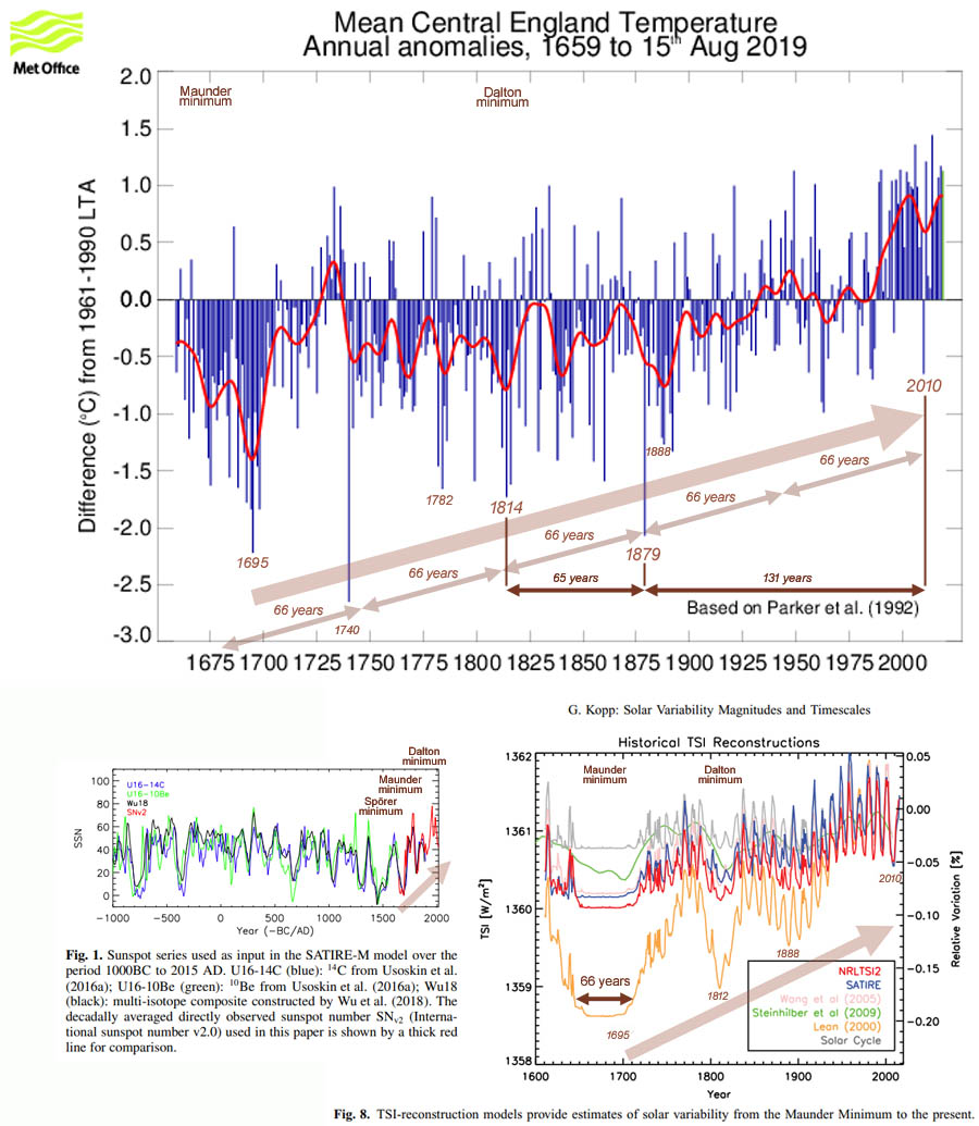
Figure 17: Upward-looking trend with five 66-year cycles in both the temperature of Central England
and the total solar irradiance39,40,41.
In the scientific literature, a cycle of 66 years has now been associated with, among other things: the Atlantic Multidecadal Oscillation (AMO)42, Moesson rainfall patterns19, icecores43 and the 11-year sunspot cycle19,22,23. Also, the 66-year cycle can get connected with six oscillations of the 11-year sunspot cycle. The phenomenon of the Yoshimura cycle can also be taken into consideration; it was defined by Yoshimura in 1979 as a 55-year cycle that related to the sunspot cycle and is associated with the magnetic oscillation of the sun. Prior to the description of Yoshimura, the assumption used to be made that it involved a 88-year cycle44.
It is also established that when making estimates with regard to global warming over the past decades, account must be taken of the possibility that various natural factors might have made a significant contribution:
• Part of the warming of the ocean system is created through the mantle of the Earth's crust via: volcanism, hydrothermal springs and geothermal springs. According to empirical measurements, the frequency of major earthquakes in categories 6 and 7 has increased in the last 50 years; however, this is largely regarded by experts as an artifact due to better measurements45.
• The relationship between El Nino and global warming is not well understood yet. A NASA employee has described that the contribution of El Nino in 2016 amounted to around 25% of the warming since the start of the industrial revolution. It is also clear that El Nino has contributed to rising temperatures in the atmosphere. However, at the same time it is assumed that El Nino's net effect creates a cooling of the ocean system. Moreover, the experts believe that the heat content of the ocean system is a much more reliable indicator of 'global warming'. With regard to this last point, it should be noted that at the same time there is still much uncertainty about the heat content of the deep sea. For example, at the beginning of 2019 researchers described that the deep sea is cooled down in the past centuries, and compensated for about 1/4 of the warming of the ocean low above 2000 meters46. There are also indications that a positive phase of the Indian Ocean might play an important role in the formation of 'super El Ninos'.
• Natural variability within both the ocean system and vegetation are factors that also play a role in global warming. For example, there is still great uncertainty about the percentage of anthropogenic CO2 that disappears into the ocean and the percentage that disappears into vegetation on land. According the NOAA approximately 50% of the anthropogenic CO2 remains in the atmosphere and approximately 25% disappears in the ocean and 25% in the vegetation; however, estimates have also been made in the past where 20-40% may disappear in the ocean and 5-30% in vegetation47. In addition, speculative estimates have also been made based on raw CO2 values where the increase in CO2 in the atmosphere over a period of 33 years is only for 1.5% attributed to anthropogenic emissions and 2.3% to warming in the ocean system48.
• Another factor concerns the decrease of phosphates in the atmosphere worldwide since the 1980s; 'brightening' has made a direct contribution to the warming of the ocean system. KNMI acknowledges, for example, that in Europe since 1976 cleaner air has contributed 10-20% of the warming; in Eastern Europe the contribution is even much larger at 50%49.
• After correction for natural variation, a study from 2016 also referred for the first time to a 'break' (read: gap) in the growth of CO2 in the atmosphere50. This concerns the period 2002-2014 in which the annual increase in CO2 in the atmosphere showed a downward trend - which was subsequently broken by a record increase in 2015. After the '15/'16 super El Nino ended, annual growth fell back in 2017 and 2018 to levels that were surpassed in some years during the 'pause' - see figure 9. The introduction already mentioned that the ocean has been responsible for up to 40% of the variability of CO2 in the atmosphere in recent decades; climate models also hardly take this natural factor into account.
The heat absorbing capacity of CO2 as a greenhouse gas does not apply to CO2 absorbed by the ocean system42. According to the greenhouse theory, the warming of the ocean system is mainly caused by the warming of the atmosphere. However, the atmosphere is on average cooler than the earth's surface; for example, the average temperature of the surface water is around 17°C, which is more than 2°C warmer than the average temperature in the atmosphere in which we live - which is currently estimated at around 14.7°C. The greenhouse theory therefore seems to contradict the 2nd law of thermodynamics, which describes:
'Er is geen proces mogelijk dat als enige gevolg heeft dat warmte van een voorwerp met lage temperatuur naar een voorwerp met een hogere temperatuur stroomt'.
[No process is possible that has the sole consequence that heat flows from a low temperature object to a higher temperature object]
There is still much uncertainty about the impact of clouds in the climate system on Earth, but the cloud system does not work like a glass roof like is seen in the case with a greenhouse; many descriptions of the greenhouse effect theory appear to be based on reasoning that contradicts various laws of thermodynamics and physics51.
The complex relationship between temperature and CO2 is characterized by complementary feedback mechanisms; in most perspectives the relationship between temperature and CO2 is characterized by a dynamic that is accompanied by a counter-phase, or a negative forcing:
- In the daily cycle, CO2 is in an opposite phase and also in a delay relative to temperature (with vegetation in between). During the day the temperature is high and the CO2 level in the atmosphere is then relatively low, because CO2 is then being absorbed by the vegetation to establish growth with with solar radiation and water, while at night the vegetation excretes the CO2 because growth is then hardly possible due to a lack of solar radiation. In addition to the opposite phase with temperature, CO2 is also in an opposite phase with respect to both solar radiation, air pressure, wind speed and also with ozone52.
- Also, in the seasonal cycle, CO2 is in an opposite phase and also in a delay relative to temperature (with the vegetation and ocean in between). In the summer season the temperature is high and CO2 is converted during the growth of vegetation, with the result that at the end of the summer the CO2 level in the atmosphere reaches the lowest level within the seasonal cycle. Subsequently, in the course of autumn and winter, the CO2 is excreted again as the seasonal vegetation dies (with leaves falling from the trees and flowers losing their fruits). Incidentally, during the summer season the water from both the oceans, the lakes and the rivers is less able to absorb CO2 because of the higher temperature; during the winter season, these systems absorb a relatively large amount of CO2. So there is also an opposite phase between the seasonal vegetation and the H2O cycle52.
- In the perspective of the ice age cycle, CO2 follows the temperature with a delay that can vary in the order of hundreds of years (through the intervention of the ocean system), where CO2 is recognized as not much more than one of the many factors in internal feedback of the climate system53.
It is also relevant for this perspective that, according to KNMI fog and mist (both can be recognized as a form of low-hanging clouds) provide a cooling effect both during the day and at night; From this it can be deduced directly that the presence of water vapor at low altitude is likely to cause negative feedback in the climate system. Low-hanging clouds only cool off during the day (because solar radiation is blocked). At night, low clouds ensure that heat emitted by the earth's surface is retained for longer. Generally speaking, high clouds are said to contribute to global warming. For the clouds system as a whole,NASA describes that it provides approximately -5°C cooling for the earth. The climate brochure from the Dutch KNAW shows that the net impact of clouds is considered to be one of the most controversial topics in the scientific climate debate.
The analysis at the level of individual years has led to two changed insights compared to the analysis at the level of the decades that was presented for the HadCRUT4 temperature series in june 2019:
1 - There is a 66-year cycle (previously it was named a 70-year cycle).
2 - The 66-year cycle shows an amplitude of 0.12°C (previously it was referred to as an amplitude of at least 0.125°C). It can also be mentioned here that based on Fourier analysis in a 2012 study it was concluded that in the perspective of the multidecadal cycle an amplitude is possible up to 0.17°C14.
The conclusion is that the definition for climate needs a re-definition, because the 30-year period currently being used to study climate change can also be held responsible for the overestimation of various trends, including: the structural impact of global warming and the correlation between the temperature with CO2 observed in the decades after the 1970s. The upward phase of the 66-year cycle is a phenomenon that is part of natural variability. The impact of this phenomenon has not been taken into account in the projection of the IPCC for the year 2100. The result is that the warming expected by the IPCC (estimated at +0.20deg;C per decade for the of the first half of the 21st century) is overestimated with about a factor of 2 compared to the average structural upward trend of +0.09°C per decade. Logically, the same factor 2 is probably also indicative for the overestimation with regard to the impact of CO2.
After the August 12 publication on KlimaatCyclus.nl, this article was subsequently also presented on August 26 on Climategate.nl; the discussion that has arisen on the Climategate platform has lead to the 5 additional comments below:
• The 66-year cycle is based on a natural mechanism, variations are therefore possible within a limited bandwidth. The concept of the 66-year cycle does include a likewise bandwidth like it is for example found in: the 11-year solar cycle (bandwidth: 9-14 years) and the 5-year ENSO cycle (bandwidth: 2-7 years). Based on Figure 1 combined with the influence of the sunspot cycle and the ENSO cycle, the estimate can be made that the 66-year cycle has a bandwidth that might not be much greater than 65-69 years.
• 2 - An additional calculation has been made for the trend in the warming on top of the 66-year cycle based entirely on quantitative data for respectively: figure 3 (+0.088°C per decade), figure 12 (+0.086°C per decade) and figure 13 (+0.101°C per decade); despite the fact that these values show a limited deviation from the associated qualitative trends, the average of the three quantitative trends exactly matches the average trend calculated in paragraph X based on six trend values. Also, the results based on the quantitative data for the two variants of the 66-year cycle described in figure 3 and figure 12 show that after the correction made (aimed at getting rid of the slope in the cycle) in both cases the upward slope is disappeared completely; in figure 3 there is a small over-correction, which logically could have lowered the upward trend of the perspective shown in figure 3 a little further in the direction of the quantitative result for warming up on top of the 66-year cycle.
• 3 - The straight pink line in figure 6 is the result of the logarithmic scale on the X-axis. In the article, the pink trend line in figure 6 has remained entirely undisputed; figure 6 has also played no role in the analysis apart from the fact that the correlation in figure 6 and figure 7A have about the same magnitude. In figure 7 all four graphs are presented with a normal scale on the X-axis; if a trend line were to be added to these graphs, it would have shown a logarithmic curvature.
• 4 - From the overestimation that applies to both the trend of the temperature rise and the corresponding estimate for the impact of CO2, it can be concluded that the overestimation also applies to the trend of the annual growth of CO2 (this point involves figure 9, though the illustration does not describes any trend and it is also not discussed inside the article).
• 5 - The final section 'X Discussion & conclusion' includes a reference to controversial assumptions regarding aerosols that are being used in field of climate science. This mainly concerns the role of aerosols in the troposphere where the uncertainty especially relates to the role that aerosols play in cloud formation. There is considerably less uncertainty about the impact of aerosols in the higher stratosphere, where there are no clouds.
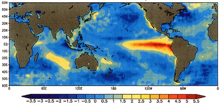

References:
1 - Change detection in hydrological records - a review of the methodology - W. Kundezewicz & A. Robson (february 2004)
2 - KNMI: Future Weather, (2012); page 9 describes: "Generally such a climatological period is defined as a 30-years period, although we note that even 30 years may be too short to capture all natural climate variability."
3 - KNMI'14: Klimaat Scenarios voor Nederland (2014); page 6 describes: "De twee kolommen met waarnemingen laten zien dat de toename in de winterneerslag over 30 jaar ongeveer even groot is geweest als de natuurlijke variaties gemiddeld over 30 jaar", page 8: "Hoe langer de periode waarvoor een gemiddelde wordt berekend, hoe kleiner de invloed van natuurlijke variaties op dit gemiddelde is. Maar zelfs gemiddelden over 30 jaar - het ijkpunt van wat als normaal weer wordt gezien - zijn erdoor beïnvloed (zie figuur 1). Vooral voor neerslag en wind zijn natuurlijke variaties in gemiddelden over 30 jaar aanzienlijk vergeleken met de veranderingen in de 30-jaar gemiddelden volgens de klimaatscenario's." [The two observation columns show that the 30-year increase in wintertime returns has been about the same as the 30-year average natural variations", page 8: "The longer the period for which an average is calculated, the less the influence of natural variations on this average. But even averages over 30 years - the benchmark for what is considered normal weather - are affected by it (see figure 1). Especially for precipitation and wind, natural variations in averages over 30 years are considerable compared to the changes in the 30-year averages according to the climate scenarios.]
4 - KNMI: Wereldgemiddelde temperatuur en CO2 nemen verder toe (november 2018); "Dit kwam in 2015 en 2016 grotendeels door een sterke El Nino, die de wereldgemiddelde temperatuur even boven de trendlijn optilt." [This was largely due to a strong El Nino in 2015 and 2016, which raises the world average temperature just above the trend line.]
5 - CarbonBrief - Interactive: How much does El Nino affect global temperature? (january 2017)
6 - New study explains unusual 2015/16 El Nino heat budget - M. Mayer et al. (april 2018)
7 - NASA: Sheet 2: "Net impact of El Nino on the global carbon cycle is an increase in atmospheric CO2 concentrations" - A. Chatterjee et al., (march 2018)
8 - Analysis of Temporal Signals of Climate - P. Stallinga & I. Khmelinskii (october 2018)
9 - A successful prediction of the record CO2 rise associated with the 2015/2016 El Nino - R.A. Betts (november 2018)
10 - The unstable CO2 feedback cycle on ocean planets - D. Kitzmann et al. (august 2015)
11 - Greenhouse gas growth rates - J. Hansen & M. Sato (september 2004); source describes 14% for period 1850-2003, adjusted for 1850-2018, percentage rises to 15%
12 - Decadal trends in the ocean carbon sink - T. DeVries (may 2019)
13 - KNMI: Klimaatfluctuaties (february 2019)
14 - Fourier analysis of measurements and Earth System Model simulations - S. Henriksson (october 2012)
15 - The carbon cycle response to two El Nino types: an observational study - P. Chylek et al. (january 2018); figure 4: CO2 is 7 to 8 months behind the temperature
16 - Variations in atmospheric CO2 growth rates coupled with tropical temperature - W. Wang et al. (augustus 2013)
17 - State of the climate 2018 - O. Humlum (april 2019)
18 - Global lake response to the recent warming hiatus - L.A. Winslow et al. (march 2018)
19 - Solar Variation and Climate Change - in reference to Indian Rainfall Pattern
- V.K. Pandey & A. Mishra (2015)
20 - Solar Minima, Earth's rotation and Little Ice Ages in the past and in the future: The North Atlantic-European case - M.A. Mörner (january 2010)
21 - On the time-varying trend in global-mean surface temperature - Z. Wu et al. (july 2011)
22 - Multi-scale harmonic model for solar and climate cyclical variation throughout the
Holocene based on Jupiter-Saturn tidal frequencies plus the 11-year solar dynamo cycle
- N. Scafeta (2012)
23 - The predicted size of cycle 23 based on the inferred three-cycle
quasi-periodicity of the planetary index Ap - H.S. Ahluwalia (june 1998)
24 - Wikipedia: "Het klimaat is de gemiddelde weerstoestand (temperatuur, windkracht, bedekkingsgraad en neerslag) over een periode van minimaal 30 jaar." [The climate is the average weather condition (temperature, wind force, coverage and precipitation) over a period of at least 30 years]
25 - Natural Climate Oscillations may Counteract Red Sea Warming Over the Coming Decades - G. Krokos (march 2019)
26 - A Significant Component of Unforced Multidecadal Variability in the Recent Acceleration of Global Warming - T. Delsole (february 2011)
27 - Recent developments in studies of climate since A.D. 1500 - R.S. Bradley & P.D. Jones (1995)
28 - Compendium voor de Leefomgeving: Temperatuur in Nederland en mondiaal, 1906 - 2017 (april 2018)
29 - KNMI: Poolklimaat verandert het snelst
30 - Decadal-scale progression of Dansgaard-Oeschger warming events - Erhardt et al. (december 2018); citaat: "In the course of the last glacial period, ice-core records from Greenland reveal millennial-scale warming episodes, called Dansgaard-Oeschger (DO) events (Dansgaard et al., 1993; NGRIP project members, 2004). During their onset, temperatures
in Greenland increased rapidly by 10-15 °C from cold stadial (GS, Greenland Stadial) to warmer interstadial (GI, Greenland
20 Interstadial) conditions within a few decades (Kindler et al., 2014; Huber et al., 2006; Severinghaus, 1999), going along with an
almost doubling of the local snow accumulation (Andersen et al., 2006)."
31 - Moho and basement depth in the NE Atlantic Ocean based on seismic refraction data and receiver functions - Funk et al. (july 2016)
32 - The recent warming on Svalbard and its relation to atmospheric circulation and sea ice cover (sheet 7) - Isaksen et al. (november 2017)
33 - De Toestand van het Klimaat - De Noord Atlantische Oscillatie - G.P. Können et al. (1999)
34 - Black Box Identification of Earth's Climate System - P. de Larminat (july 2019)
35 - The Politically Incorrect Guide to Climate Change - M. Morana (2018)
36 - Multi-periodic climate dynamics: spectral analysis of long-term
instrumental and proxy temperature records - H.-J. Lüdecke et al. (february 2013)
37 - Paleoclimate forcing by the solar De Vries/Suess cycle - H.-J. Lüdecke et al. (february 2015)
38 - Redefining the limit dates for the Maunder Minimum - J.M. Vaquearo & R.M. Trigo (2015)
39 - Hadley Centre Central England Temperature (HadCET) dataset (august 2019)
40 - Magnitudes and timescales of total solar irradiance variability - G. Kopp, figure 8 (june 2016)
41 - Solar total and spectral irradiance reconstruction over the last 9000 years
- C.-J. Wu et al, figuur 1 (november 2018)
42 - High-frequency cyclicity in the Mediterranean Messinian
evaporites: evidence for solar-lunar climate forcing - V. Manzi et al. (2012, figure 9a)
43 - 8,000 years of AMO? - G. Foster (march 2011)
44 - The solar-cycle period-amplitude relation as evidence of hysteresis of the solar-cycle nonlinear magnetic oscillation and the long-term (55 years) cyclic modulation - H. Yoshimura (february 1979)
45 - Evidence of Variable Earth-heat Production, Global
Non-anthropogenic Climate Change, and Geoengineered Global Warming and Polar Melting - J.M. Herndon (april 2017)
46 - The Little Ice Age and 20th-century deep Pacific cooling - G. Gebbie & P. Huybers (january 2019)
47 - CARBOSCHOOLS: Wat we weten Wat we niet weten En hoe we proberen de wereldwijde milieuveranderingen beter te begrijpen: Een inleiding op onderzoeksvragen, uitdagingen en uitvoering voor 'CarboSchools' projecten (2006)
48 - Oceans, Ice & Snow and CO2 Rise, Swing and Seasonal Fluctuation - M.D. Nelson & D.B. Nelson (october 2016)
49 - KNMI: Mist en nevel afname in Europa (october 2009); citaat: "We schatten aan de hand van het temperatuureffect van figuur 3 en de afname van figuur 2 dat de afname van mist en nevel 10%-20% aan de opwarming van de dagtemperatuur heeft bijgedragen. In Oost-Europa is de bijdrage veel groter, tot 50%." [Based on the temperature effect of Figure 3 and the decrease in Figure 2, we estimate that the decrease in mist and mist contributed 10% -20% to the warming of the day temperature. The contribution is much larger in Eastern Europe, up to 50%.]
50 - Recent pause in the growth rate of atmospheric CO2 due to enhanced terrestrial carbon uptake - T.F. Keenan et al. (november 2016)
51 - Role of greenhouse gases in climate change - M. Hertzberg et al. (2017)
52 - Seasonal and Diurnal CO2 Patterns at Diekirch, LU 2003 - 2005 - F. Massen et al. (march 2007); section 4.1 & 4.3
53 - Breakpoint lead-lag analysis of the last deglacial climate change and
atmospheric CO2 concentration on global and hemispheric scales, LU 2003 - 2005 - Zhi Liu et al. (may 2018)
CLIMATE INDEX:
•
Millennium analysis: climate sensitivity CO2 is below IPCC bandwidth
•
IPCC dataset sun explains half of warming since 1815
•
Impact sun on climate is underestimated significantly
•
Since 17th century: +1,1 °C by sun
• 1890-1976: Sun shows perfection correlation with temperature
• Side-role for CO2: solar activity explains warming since 1976
• Impact of CO2 on climate overestimated (substantially) due to 66-year cycle & El Nino
What do proxy climate indicators show?
• 2° Institute proxies: temperature rose in the past multiple decennia in a row even faster
• PAGES 2k Network illustration (2013)
• PAGES 2k Network illustration: 2019 hockeystick graphic vs 2013 temperature data
ClimateCycle articles in Dutch language:
•
IPCC dataset zon verklaart met vulkanisme helft opwarming sinds 1815
•
Tussen 1685 en 1976 volgde de temperatuur de totale zonnestraling
• Boekrecensie: SOLAR MAGNETIC VARIABILITY AND CLIMATE
•
Online seminar door zonnefysicus Dr. Greg Kopp: 'Zonnestraling & klimaat'
•
Impact zon op klimaat fors onderschat
•
Sinds 17de eeuw: +1,1 °C door zon
•
SAMENVATTING: Hoe ontstaat de Klimaatcyclus en wat is haar impact?
• 1890-1976: Zon toont perfecte correlatie met temperatuur
• Zon verklaart opwarming sinds 1976
• El Nino & 66-jarige cyclus: CO2 overschat
• 70-Jarige cyclus: opwarming overschat
• Global warming vs fluctuaties in 2 dagen
• Oceaan: diepzee koelt af
• KlimaatCyclus.nl