|

June 26, 2020

22-year magnetic solar cycle [Hale cycle] responsible for significant underestimation of sun's role in global warming but ignored in climate science

Martijn van Mensvoort

Abstract

Reconstructions for global temperature development show an upward oscillation for the period of the 1880s through 1980s. This oscillation is being associated with natural variability and the temperature rise between the 1910s and 1940s with increased solar activity.
The temperature impact of the 11-year solar cycle [Schwabe cycle] and the physical mechanism involved are insufficiently understood. Here, for the 22-year magnetic solar cycle [Hale cycle] a seawater surface temperature impact is described of 0,215 °C (0,238 ± 0,05 °C per W/m2); the impact is smaller for the 11-year cycle: 0,122 °C (0,135 ± 0,03 °C per W/m2). A parallel development is described for seawater surface temperature [HadSST3] and the minima of total solar irradiance [LISIRD TSI] after a correction based on the 22-year cycle. The correction involves two categories of solar minima: (1) primary minima form in the phase with magnetic poles in the original position and (2) secondary minima form in the phase when the poles have switched positions.
With the correction, the combination of the primary and secondary minima shows for the period 1890-1985 a high solar sensitivity: 1,143 ± 0,23 °C per W/m2 (declared variance: 91%). The impact of long-term solar fluctuations is 4,8x larger than during the short-term course of the 22-year cycle and 8,4x larger than during the 11-year cycle. This implies that the sun has caused a warming of 1,07 °C between the Maunder minimum (late 17th century) and the most recent solar minimum year 2017 - well over half of the intermediate temperature rise of approximately 1,5 °C.
The results demonstrate that the 22-year cycle is a crucial factor in order to better understand the relation between solar activity & temperature development. Ignoring both the 22-year cycle and the amplifying factor for the TSI signal at the top of the atmosphere leads to significant underestimation of the sun's influence in climate change combined with an overestimation of the impact of anthropogenic factors and greenhouse gases such as CO2.

---

CONTENT

Abstract
Introduction
Results

• Total solar irradiance (TSI) & temperature correlate higher during minima than during maxima
• Temperature profile for the 22-year & 11-year solar cycle
• Primary and secondary TSI minima show high correlation with seawater surface temperature
• Multi-year TSI minima show a comparable trend with seawater surface temperature after correction

Discussion & Conclusion
Method
References

---

Introduction

In a 2006 Dutch scientific report by the Royal Netherlands Meteorological Institute (KNMI) in collaboration with the NIOZ, is reported that prior to 1950 the influence of humans on temperature had been negligible¹. This makes the period prior to 1950 ideally suited to study the influence of the sun on temperature.
In the current research, the influence of the sun on seawater surface temperature is being studied for the period 1890-1985. This timeframe includes 3 periods in which the temperature trend has changed direction and it includes a total of 10 solar minimum years. According to experts, prior to 1880 insufficient data is available for a reliable estimate of the global seawater surface temperature; only after the year 1950 did the uncertainty margin decrease to a low level for most regions of the world². Also of importance, among experts there is consensus regarding that the heat content of the ocean system is probably the best indicator of global warming ³; logically, the warming of the seawater surface temperature is therefore probably a more relevant indicator than the warming of the atmosphere. In this study the HadSST3 dataset is used for seawater surface temperature.

There is controversy about the influence of the sun on the climate involving a wide range of aspects. Estimates for the temperature effect of the 11-year solar cycle [Schwabe cycle] vary from less than 0,05 °C (barely recordable)¹ to more than 0,25 °C⁴. However, for the same amount of energy a much larger temperature effect is expected in the longer term. For a 200-year cycle, the temperature effect is 2 to 4 times larger than for the 11-year cycle, in particular due to the accumulation of energy within the ocean system¹; for even longer periods the impact is even 5 to 10 times larger^5,6.
The controversy also concerns the share of the sun in the ~0,8 °C warming in the 20th century: available estimates range from 7% (0,056 °C) to 44-64% (0,35-0,51 °C)⁷. The compilation of the historical dataset for total solar irradiance [TSI] is an important part of the controversy as well⁸. Since the 1990s, even scientific legitimacy has been debated in relation to the method used by research groups involved; among experts this issue is known as the ACRIM-PMOD controversy⁹. Large differences of opinion have arisen with regard to the TSI construction method. The widely used method of Lean et al. (1995)¹⁰ is based on 2 magnetic components and produces a curve which shows the highest TSI values in the late 1950s; while, for example, the method of Hoyt & Schatten (1993)¹¹ is based on 5 magnetic components and produces a curve which shows the highest TSI values only near the beginning of the 21st century. This explains why estimates for the influence of the sun on the climate differ both numerically and fundamentally to a great extent; numerically, the controversy involves impact differences close to a factor of 10.

In climate science the influence of the sun is studied, among other things, by means of the 11-year solar cycle. However, fundamentally, it has been established since the beginning of the last century that the 22-year magnetic solar cycle [Hale cycle] forms the origin of the 11-year sunspotscycle¹². This is important because two consecutive 11-year cycles exhibit structural differences; an example for this involves the Gnevyshev-Ohl rule¹³, which relates to the number of sunspots between 2 consecutive maximums.
It is therefore remarkable that the 22-year cycle hardly plays a role in climate science. IPCC reports do not even bother to mention the existence of the 22-year Hale cycle¹⁴. Descriptions elsewhere in the scientific literature indicate that it is probably being presumed that the manifestations of the 22-year cycle are not sensitive to the polarity change; however, the foundation of such assumptions is unclear. Because in 2008, for example, it has been determined that since the Maunder minimum the coldest phase of the 22-year cycle takes place (under the influence of cosmic rays) during the minima that occur when the polarity is positive; the magnetic solar poles are then located in their original position¹⁵.

This study therefore distinguishes between two categories of solar minima: (1) primary minima, which arise during the phase where the magnetic polarity is positive with the poles in the original position; and (2) the secondary minima, which arise during the phase where the magnetic polarity is negative and the poles have switched positions. This is crucial because trend analyzes focusing on the impact of the radiant forcing of the sun are usually based on solar minimum years, for, the phase of the solar cycle must be taken into account. The main reason for this is that the minima are both "more stable" and "more relevant" than the maxima¹⁴. In terms of the physical processes this is explained by the fact that the number of sunspots and flares is relatively small during the minima; this concerns the two magnetic components in the Lean method, which represent also the basis of the LISIRD TSI dataset used in this study. This is because the maxima are accompanied by relatively large fluctuations, which exhibit higher uncertainty than the minima. This is because the result at the maxima depends more strongly on the magnetic components used in the reconstruction than at the minima^10,11. This also explains the relevance of the choice made in this study to use the perspective of the solar minimum years as the most important point of reference for studying the climate impact of the 22-year magnetic solar cycle.

---

Results

Here the LISIRD TSI dataset¹⁶ is used; this is not an "official" TSI, but in the eyes of the author (LASP principal investigator Dr. Greg Kopp) this dataset does contain the best values available to the experts. For the pre-satellite era, the LISIRD uses the SATIRE-T TSI dataset with some "refinements"¹⁷ and for the satellite era (from 1978) the LISIRD is based on the Community Consensus TSI Composite¹⁸. For the seawater surface temperature, the HadSST3 dataset from the Hadley Center is used¹⁹.

With the Hale cycle taken in consideration, the correlations between the TSI and the seawater surface temperature are described first. The period around the minimum years 1890 to 1985 is then used in order to calculate the temperature profile for the 22-year Hale cycle (+ the temperature profile for the 11-year Schwabe cycle). Based on the minimum years, a description is then given for the solar sensitivity in the long-term perspective. A distinction is made between: (1) primary minima created during the phase with the magnetic poles in the original position; (2) secondary minima created during the phase when the poles have switched positions.

• Total solar irradiance (TSI) & temperature correlate higher during minima than during maxima

Figure 1 describes a stable correlation (r = 0,42) for the TSI and seawater surface temperature showing the same magnitude for both the period 1890-1985 and the period 1880-2018. However, for both the minimum and maximum of the solar cycle the correlations are at a significantly higher level; in accordance with the expectation¹⁵, the impact of the effect for the individual phases is largest at the minima.

Moreover, the correlations at both the primary & secondary minima and the primary & secondary maxima reach an even higher level. For the period 1880-1985, very high correlations with almost the same value are found for both the primary and secondary minima. And for the primary and secondary maxima the same correlation value is found. This shows that during the course of the 22-year cycle, the fluctuation of the TSI-temperature correlation shows a high degree of regularity.

The structurally higher correlations in the primary and secondary minima series (compared to the combination of both series) are related to the Gnevyshev-Ohl rule; using the dashed green curves the impact is shown in figure 1 for both the TSI minimums and the TSI maximums.

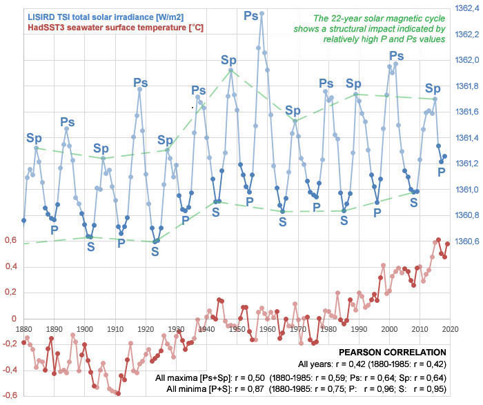
Figure 1: The individual phases of the solar cycle show correlations for the LISIRD TSI total solar irradiance and HadSST3 seawater surface temperature that are significantly higher compared to the values for the entire cycle. In addition, the minima show structurally higher correlation values with respect to the maxima. The TSI has a structural impact due to the 22-year magnetic solar cycle, which is expressed in relatively high primary TSI minima (P) and maxima (Ps); this structural phenomenon is in accordance with the Gnevyshev-Ohl rule, which in literature is being related to only the maxima of the sunspot cycle¹³.

---

• Temperature profile for the 22-year & 11-year solar cycle

The HadSST3 seawater surface temperature profile for the 22-year solar cycle has been determined based on the period 1882-1988. This period includes: 5 secondary maximums, 5 primary minimums, 5 primary maximums, and 5 secondary minimums; the mean values are being used to serve as a separate reference point. The average value is then determined for the years around each of these 4 reference points. This results in 4 reference profiles that each show a temperature difference within the range of 0,20-0,27 °C within 7 to at most 11 years with an average value of 0,236 °C. The trend has subsequently been removed from each of the 4 reference profiles. Finally, the temperature profile was compiled with the years immediately around 4 reference points. In particular the years around the minimum reference points have been used for this because the years around the two maximum reference points show less consistency compared to the other 3 reference profiles (the method section describes the procedure used in detail). The profile for the 11-year Schwabe cycle is entirely based on the profile of the Hale cycle; here only the minima of the Hale profile acted as a reference point.

The temperature profile for the Hale cycle is shown in figure 2. The length of the Hale profile is only 21 years because the Hale cycles in this period were relatively short on average: the average length of the Hale cycles in the period 1890-1985 is approximately 21 years. Within the Hale cycle profile, the largest temperature difference is found between the primary minimum and the phase that follows 8 years after the primary minima. The temperature difference between and the primary minimum the temperature peak is 0,215 °C. The temperature difference between the primary minimum and the secondary minimum is 0,059 °C. By the way, the TSI primary maximum occurs here 4 years after the TSI primary minimum and the TSI secondary maximum occurs 5 years after the TSI secondary minimum. The TSI secondary maximum coincides with the highest temperature value in the 2nd part of the Hale cycle (starting from the secondary minimum and ending at the primary minimum).

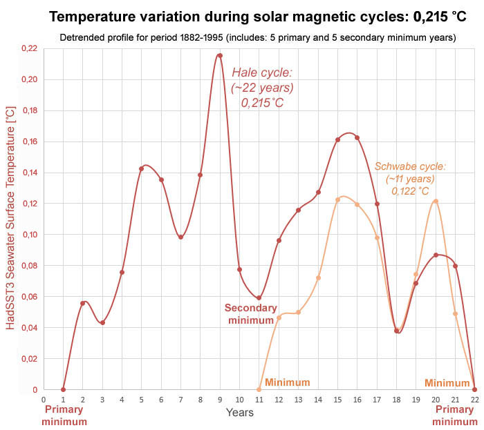
Figure 2: The seawater surface temperature profile for the Hale cycle based on the period 1882-1988 (which includes 5 primary minima and 5 secondary minima) shows a maximum impact for the of 0,215 °C. During the first part of the Hale cycle, the fluctuations greater than during the second part. The temperature profile for the Schwabe cycle shows a maximum impact for the seawater surface temperature of only 0,122 °C.

Figure 2 shows that the first part and the second part of the Hale cycle show an asymmetrical temperature trend; during the first part, the fluctuations are more frequent and the amplitude is higher compared to the second part. The temperature peaks relatively late in the first part and peaks relatively early in the second part. In addition, the profile of the Hale cycle shows an oscillation with fluctuations that take 2 to 7 years, which corresponds exactly to the variation described for the duration of the ENSO cycle; this is not entirely surprising as it is known that there are strong statistical relationships between ENSO and the activity of the sun²⁰.

For the period 1882-1988, the radiative forcing between all adjacent maxima and minima shows an average value of 0,86 W/m2. Combined with the average maximum temperature difference within the profile of 0,215 °C this results in a solar sensitivity within the Hale cycle of 0,25 °C per W/m2 at the top of the atmosphere (TOA); converted to the surface of the earth, this results in a value of 1,43 °C per W/m2 (via a conversion factor of 0,175: 25% based on the spherical formation of the earth in combination with 70% albedo). However, the impact of an amplifying factor for the TSI signal from the sun at the top of the atmosphere has not yet been taken into account; in the section discussion & conclusion a amplification factor with a value of 6x is used to find the solar sensitivity for the Hale cycle on the earth's surface, which results in a value of 0,238 °C per W/m2. For the 11-year cycle, a considerably lower solar sensitivity is found on the earth's surface: 0,135 °C per W/m2. Within the conceptual framework of the IPCC, both the 22-year Hale cycle and the amplification factor are being ignored¹⁴.

For the sake of completeness, figure 2 also shows the temperature profile for the 11-year Schwabe cycle (which has been derived directly from the Hale cycle profile). A striking feature of the profile for the Schwabe cycle is that it contains 2 peaks; this is in line with the fact that for the 11-year sunspot cycle 2 maxima have also been described which arise in a time frame of 2 to 4 years. The literature describes that the first peak is related to UV radiation and the second peak is related to geomagnetic disturbances (+ aurora phenomena)²¹.

---

• Primary and secondary TSI minima show high correlation with seawater surface temperature

The upper part of figure 3 describes for the period 1890-1985 a high correlation for TSI and seawater surface temperature with a declared variance of 91% for both the primary and secondary minima. This involves the same correlations that are described for the minima in figure 1; however, in figure 3 the TSI scale has been adjusted to show the dynamics visually. For both minima perspectives separately, the temperature follows the trend of the TSI, with exception for the first transition of the secondary minima where both factors move in opposite directions.
It is striking that when the distinction between the primary and secondary minima is not made 6 of the 9 transitions show an opposite movement between the TSI and the temperature. This dynamic for the combination is clearly inconsistent with the dynamic at the primary and secondary minima separately.

The introduction section has described that temperature during the minima of the primary phase reaches the lowest level since the Maunder minimum. Regarding the physical mechanism involved is known that during the negative phase of the solar cycle the supply of cosmic rays (which is associated with cloud formation²²) is more sensitive because the supply comes then more via the equator of the sun, while during the positive phase the supply comes more via the poles¹⁵. This implies that based on the direction of supply of cosmic rays it can be stated that the relationship between TSI and temperature directly depends on the polarity of the sun. During the negative phase (which starts around the primary maximum, during the transition from the primary minimum to the secondary minimum) a relatively small amount of energy is needed for a temperature increase, while during the positive phase (which starts around the secondary maximum, during the transition from the secondary minimum to the primary minimum) more energy is required for the same temperature rise. Logically this means that a structural correction is needed to describe and better understand the relationship between the TSI and the temperature - although the use of a correction is by principle not necessary for a comparison between years that are in the same phase of the 22 year cycle.

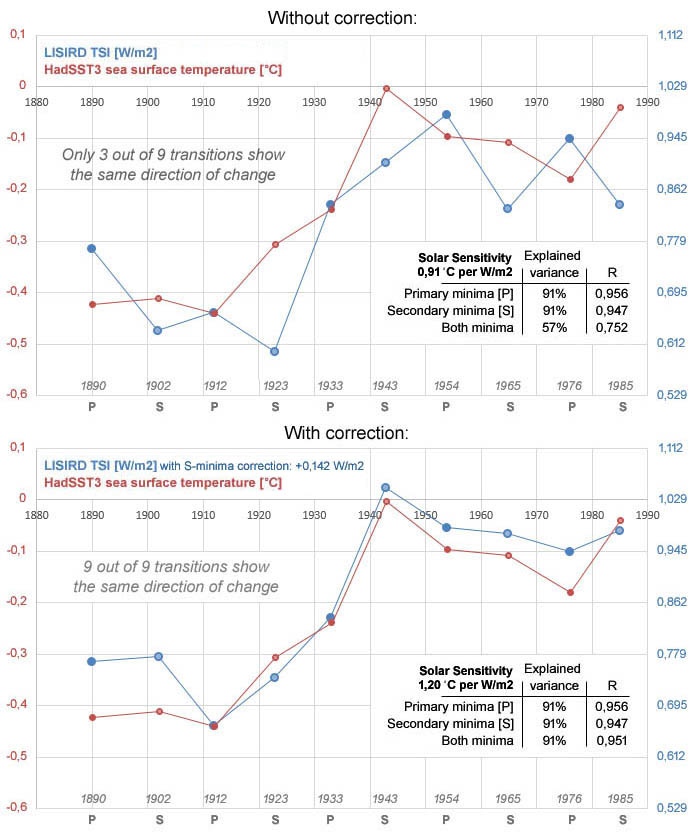
Figure 3: (top) HadSST3 seawater surface temperature plotted against the LISIRD TSI (+1360 W/m2) shows that for the period 1890-1985 very high correlations are found only at the primary and secondary minima separately; (bottom) after a correction of +0,142 W/m2 focused on the secondary TSI values, a very high correlation is also found for the combination of the minima. Using a regression analysis the solar sensitivity at the top of the atmosphere (TOA) for this period is established at: 1,20 °C per W/m2 with regard to the LISIRD TSI values above 1360 W/m2 based on a declared variance of 91%. The ratio of the scales is adjusted in order to describe the effect visualy and the values for the minimum year 1912 have been used as reference point. For the primary and secondary minima separately, the solar sensitivity (TOA) is in respective: 1,10 °C per W/m2 and 1,22 °C per W/m2, respectively. Both the top and bottom result are shown with scale ratios based on the result including the correction. The Earth's solar sensitivity yields values of the same magnitude (~95%) after taking into account corrections for the shape of the Earth (~25%), albedo (~70%) and an amplifying factor (~6x) for the TSI signal.

In the bottom part of figure 3 a correction has been applied to the secondary TSI values. The correction causes the correlation for the combination of the primary and secondary minimum values ends up at exactly the mean value of both minima separately. This result implicates that in the bottom part of figure 3 the explained variance for the combination ends up at the same high percentage of 91% as for both minima separately, while in the top part of figure 3 the explained variance is only 57%. In addition, after using the correction the TSI and temperature move in the same direction at all 9 transitions. The solar sensitivity is 1,20 °C per W/m2 at the top of the atmosphere (TOA); converted to Earth's surface this produces a value of 6,86 °C per W/m2 (via a conversion factor of 0,175: 25% based on spherical soil in combination with 70% albedo). However, this does not yet take into account the influence of an amplifying factor on the TSI signal at the top of the atmosphere; the discussion & conclusion section assumes an amplification value of 6x which results in a solar sensitivity on earth's surface that is only slightly lower than at the top of the atmosphere: 1,143 °C per W/m2.

The solar sensitivity of 1,20 C per W/m2 TOA (for Earth's surface: 1,143 C per W/m2) for the period 1890-1985 combined with the solar sensitivity during the 22-year solar cycle of 0,25 C per W/m2 TOA (for the Earth's surface: 0,238 C per W/m2) implies that the long-term solar sensitivity is 4,8x higher than during the short-term perspective of the 22-year cycle. When compared to the 11-year cycle, the long-term solar sensitivity is 8,4x higher.

According the LISIRD TSI dataset, the total solar irradiance between the Maunder minimum (1360,274 W/m2 TOA) and the most recent primary minimum year 2017 (1361,215 W/m2 TOA) has increased by 0,941 W/m2 TOA. Based on the long term solar sensitivity of 1,143 °C per W/m2 after taking into account the shape of the earth (25%), albedo (70%) and the amplifying factor (6x) for the TSI signal, this results in a temperature rise at the earth's surface of 1,07 °C (based on the TSI signal of 1,20 °C per W/m2 TOA, the value is slightly higher: 1,13 °C).

The magnitude of the correction with a value of more than 0,1 W/m2 is approximately one tenth of the average fluctuation of the TSI during an 11/22 year solar cycle. This is the same order of magnitude found at the structural variations of the sunspot cycle based on the Gnevyshev-Ohl rule¹³.

---

• Multi-year TSI minima show a comparable trend with seawater surface temperature after correction

The correction method aimed at the secondary TSI minimum values has also been applied to the minimums based on the 3-year, 5-year, 7-year, 9-year and 11-year average values. Figure 4 shows that the magnitude of the correction for the 3-year to the 9-year average is slightly smaller (0,110-0,138 W/m2) than the correction value of the minimum years (0,142 W/m2), but it consistently concerns the same order of magnitude. At the 11-year average, an even smaller correction value is found (0,100 W/m2); however, because there is an overlap between various periods, the result for the 11-year period is disregarded in this analysis.

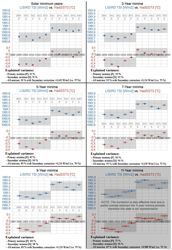
Figure 4: After applying a correction aimed at the secondary minima, the 1-year, 3-year, 5-year, 7-year and 9-year periods around the minima show a similar picture. The first 5 values of both the LISIRD TSI and the HadSST3 are lower than the last 5 values. For the first 5 values the 1912 minimum always shows the lowest value and the 1933 minimum shows the highest value; for the last 5 values the 1976 minimum always shows the lowest value.

Figure 4 shows for the 1-year to 9-year minima that the first five values of both the TSI and the seawater surface temperature are lower than the last five minima. Also, the first five values always show the lowest value at 1912 and the highest value at 1933; for the last five values the year 1976 always shows the lowest value.

Only the 1-year to 5-year minima show the same direction of the trend at all 9 transitions for the LISIRD TSI and the HadSST3 seawater surface temperature after applying the secondary correction. In the 7-year and 9-year minima, eight out of nine transitions show the same trend direction; only the transition between 1943 and 1954 shows opposite trends. Figure 1 present an explanation for this exception because the 1958 maximum (+ the immediately surrounding years) is the largest outlier in the LISIRD TSI dataset. This phenomenon also explains why in figure 4 the highest average TSI value is found at the 1954 minimum for both the 7-year and 9-year average, while the 1-year to 5-year show the highest level for both the TSI and the temperature at the 1943-value.

For the 1-year to 9-year minima, the explained variance is within the 89-93% bandwidth after applying the correction aimed at the secondary minima. As the length of the minima period increases the value of the explained variance fluctuates only a few percent from the 91% explained variance consistently found at the 1-year minima for both the primary and secondary minima, as well as for the combination of both minima after correction.

---

Discussion & Conclusion

This article investigates the sun's impact on climate with the 22-year magnetic solar cycle. The solar sensitivity is described in 3 forms: in terms of the TSI at the top of the atmosphere; this value is then converted to the earth's surface via a correction for the spherical earth (~25%) and the albedo factor (~70%); finally, it has also been corrected for an amplifying factor that increases the temperature impact of the TSI signal at the top of the atmosphere. For a calculation of the temperature impact of the sun over a certain period, it is not strictly necessary to make the conversion to the earth's surface when phase differences within the 22-year cycle are taken into account. However, this does become necessary for a description of the solar sensitivity on the earth's surface in terms of the radiative forcing; therefore, the impact of the amplification factor will now be discussed in more detail here (without going into the possible physical mechanisms involved).

Since the 1990s experts have speculated about the impact of an amplifying factor for the TSI signal from the sun at the top of the atmosphere. Literature has taken into account the possibility that the magnification of the amplification factor could theoretically vary of the order of 2x to 10x²³. However, there is no consensus about the exact size; therefore, controversy also exists on this subject. Estimates appear to depend, among other things, on the TSI dataset used²⁴. Based on 20th century data, estimates range from 2x-3x²⁴, 3x²³, 4x-6x²⁵ to 4x-8x²⁶; the IPCC recognizes that there is great uncertainty about the radiative forcing of the sun²⁴. The most detailed estimates have been described based on the 11-year solar cycle, where the values for the amplification factor are relatively high: 5x-7x²⁷ As far as is known, there are no descriptions which indicate that there are concrete reasons to assume that the magnitude of the amplifying factor for the TSI signal also fluctuates. Therefore, it is assumed here that there is a stable amplification factor with a value of 6x combined with a bandwidth of 5x-7x. This implies that the sun's sensitivity at the Earth's surface is slightly lower compared to the value measured at the top of the atmosphere. After all factors have been taken into account, the result via the chosen amplifying value (6x) amounts to 95% of TOA value; if the amplification value were slightly lower, then the surface of the earth would have almost the same value as the TSI at the top of the atmosphere (with an amplification value of 5.7x it would have almost exactly the same value). The bandwidth for the amplifying factor is used here to describe an indication for the uncertainty margin of the solar sensitivity specific to the perspective of the earth's surface after all factors have been taken into account.

For the three perspectives examined, the following values were found with regard to solar sensitivity:

• 11-year cycle:
- Solar sensitivity based on TSI at top of atmosphere [TOA]: 0,142 °C per W/m2
- Solar sensitivity converted (25% & 70%) to surface without amplifying factor: 0,81 °C per W/m2
- Sun sensitivity converted to earth surface with amplification factor (5-7x): 0,135 ± 0,03 °C per W/m2

• 22-year cycle:
- Solar sensitivity based on TSI at top of atmosphere [TOA]: 0,25 °C per W/m2
- Solar sensitivity converted (25% & 70%) to surface without amplifying factor: 1,43 °C per W/m2
- Sun sensitivity converted to earth surface with amplification factor (5-7x): 0,238 ± 0,05 °C per W/m2

• Period 1890-1985:
- Solar sensitivity based on TSI at top of atmosphere [TOA]: 1,20 °C per W/m2
- Solar sensitivity converted (25% & 70%) to surface without amplifying factor: 6,86 °C per W/m2
- Sun sensitivity converted to earth surface with amplification factor (5-7x): 1,143 ± 0,23 °C per W/m2

This overview shows that the solar sensitivity at the earth's surface depends very much on the magnitude of the amplification factor. The value of the solar sensitivity at the earth's surface increases when the amplifying factor decreases. This also applies to the albedo factor because a lower albedo value leads to a higher result when calculating the solar sensitivity for the earth's surface.

The above implies that the solar sensitivity for the long-term perspective is more than 4x (4.8x) higher than during the short-term perspective of the 22-year magnetic solar cycle; when compared with the perspective of the 11-year sunspot cycle, the value for the long-term perspective is more than 8x (8.4x) higher. These values are approximately 2x higher than the ratios between the time spans described in literature relative to the 11-year solar cycle^1,5,6. The result also confirms earlier descriptions based on periods that go further back in time which show that the temperature impact during the 22-year cycle is 78% larger than during the 11-year cycle; in a study by Scafetta & West²⁸ a 54% higher value is reported for the 22-year cycle (0,17 ± 0,06 °C per W/m2) versus the 11-year cycle (0,11 ± 0,02 °C per W/m2). The involving literature also confirms that the change of magnetic polarity plays a key role in this¹⁵.

The IPCC describes in AR5 (2013) a temperature effect for the 11-year cycle with fluctuations of the order of 0,03-0,07 °C (mean value ~0,05 °C)¹⁴; the temperature profile for the 11-year cycle in figure 2 shows fluctuations with an average value of 0,122 °C which is more than 2x higher than the description of the IPCC.

Based on long-term solar sensitivity, it has been calculated that the sun has been responsible for a temperature rise of approximately 1,1 °C since the Maunder minimum. Estimates for the total warming since the Maunder minimum are in the order of 1,5 °C²⁹. Estimates for the temperature difference between a passive and active sun are in the order of 1 °C⁵ (up to 2 °C). Since the start of the Holocene 11,700 years ago, the activity of the sun has shown that highest change between the Maunder minimum and the early 21st century³⁰. An estimate is also available which describes that the increase in solar activity since the emergence of life on Earth can explain about half to 2/3 of the temperature increase ^31,7. This series of estimates is consistent with the long-term solar sensitivity described based on the period 1890-1985.

Because the solar minima do not coincide with the start and end of the 20th century, it is not possible to make an exact calculation based on the minima for the share of the sun in the seawater surface temperature rise between 1900 and 2000 of about 0,416 °C. However, an indicative calculation can be made on the basis of the secondary minima in the period 1902-2008 (this period covers almost the entire 20th century). For the proportion of the sun, the percentage here amounts to 62,1% of the 0,671 °C warming of the seawater surface temperature between 1902 and 2008; this percentage is not far below the upper limit of 69% described by Scafetta & West for the period 1900-2005³². For the period 1890-2017 the sun provides a share of 58,2% in the warming of 0,928 °C. Both percentages are around 60% and just below the upper limit of 64% of the bandwidth described in the introduction for the global warming in the 20th century⁷.

For the 21st century, a comparison between the primary minimum years 1996 and 2017 provides a remarkable picture, because based on the solar sensitivity of 1,2 °C per W/m2 the entire temperature rise (103.6%) is explained by the sun. However, a comparison between the primary minimum years 1954 and 2017 yields a percentage of the sun that is less than half (46.4%).

From an energetic point of view, the solar sensitivity for the long-term perspective on the earth's surface with a value of 1,143 ± 0,23 °C per W/m2 presents a measure of the equilibrium climate sensitivity parameter (λ). The temperature impact of this is comparable to a climate sensitivity for the doubling of CO2 with a bandwidth of 3,38-5,08 °C (based on: 3,7 W/m2 x 1,143 ± 0,23 °C per W/m2); the midpoint of this bandwidth is at the value 4,23 °C, which is below the upper limit of the bandwidth that the IPCC applies for climate sensitivity: 1,5-4,5 °C¹⁴. A relevant comment here arises involving the period 1912-1965.

Based on the dynamics in the lower part of figure 3, the period 1912-1965 shows an almost perfect correlation (+ combined with an explained variance of 99%) between the minimum values of LISIRD TSI and HadSST3 seawater surface temperature. If the calculation had been made on the basis of the period 1912-1965, the solar sensitivity would drop from 1,20 °C per W/m2 to 1,05 °C per W/m2 (with the use of on an unchanged correction aimed at the secondary minima of 0,142 W/m2). The warming after the Maunder minimum would amount to 0,99 C based on the period 1912-1965 and the solar sensitivity would amount to 1,00 ± 0,20 °C per W/m2 based on the amplifying factor (6x). This is energetically comparable to a climate sensitivity for doubling CO2 with a bandwidth of 2,96-4,44 °C. This bandwidth corresponds to the upper side of the IPCC bandwidth. The explained variance of 99% for the 53-year period 1912-1965 offers hardly any room for influences other than the sun; this suggests that the sun is most likely responsible for the temperature trend at least until 1965. Based on the period 1912-1965 the solar sensitivity for the long-term perspective is more than 4x (4,2x) higher than the short-term perspective of the 22-year cycle and more than 7x (7,4x) higher than the short-term perspective of the 11-year cycle.

The correction shows that there is an opposite temperature effect present around the phenomenon related to the Gnevyshev-Ohl rule; moreover, the phenomenon itself applies to both the TSI maximums and the TSI minimums in the full period starting from 1880 (see figure 1).
The magnitude of the correction appears to be more or less independent of the length of the minimum period used in the calculation; the bandwidth of the correction ranges from 0,110-0,148 W/m2 for the values based on 1 to 9 year periods around the TSI minima. This means that there is a structural temperature effect that, in terms of magnitude, approximately corresponds to the average impact of the fluctuations based on the Gnevyshev-Ohl rule. The direction of the temperature effect can be explained on the basis of the sensitivity difference for the influence of cosmic rays during the positive and negative phase of the Hale cycle¹⁵. During the negative phase, the climate is more sensitive to the supply of cosmic rays than during the positive phase. The secondary minimum falls in the middle of the negative phase (see figure 5), as a result of which the influence of the loss of cosmic radiation due to the poloidal maximum is relatively large, resulting in relatively high temperatures during the secondary TSI minima. Both the mechanism involved with the temperature effect (as a result of the change of the magnetic solar poles), as well as the magnitude of the associated impact of the temperature effect, have been described by approximate.

The temperature development might be directly related to the background solar irradiance [BSI], this concerns the radiation of the sun excluding the influence of solar flares and sunspots. This involves a dynamic component on top of the base level in the signal from the sun measured at the top of the atmosphere. Uncertainty margins for the baseline (which is estimated at around 1361 W/m2 since 2008) are significantly lower than for the TSI fluctuations which arise from magnetic activity due to solar flares [T_F] and sunspots [T_S]. This might also explain why the correlation between sunspots and temperature is low; for, this does not involve the background component at all. The formula³³ below describes that the TSI [T(t)] represents the sum of the different components. The formula contains only 2 magnetic components (in accordance with the Lean¹⁰ method); a dynamic BSI component that fluctuates over time on top of the base level component [T_Q] is missing:

T(t) = T_Q + △T_F(t) + △T_S(t)

For the period 1890-1985, the LISIRD TSI dataset shows high correlations with the NRLTSI2 dataset (0,903), IPCC AR5 dataset (0,938) and Satire S&T dataset (0,944); correlations among the other 3 TSI datasets fall within the bandwidth 0,927-0,998. For the period 1985-2012, the LISIRD TSI dataset mainly shows a high correlation with the NRLTSI2 dataset (0,961) but lower correlations are found with the IPCC AR5 dataset (0,846) and Satire S&T dataset (0,868); correlations among the other 3 TSI datasets fall within the bandwidth 0,941-0,984. For the entire period 1890-2012, the LISIRD also shows comparable correlations with the other datasets (0,916-0,926); correlations among the other 3 TSI datasets fall within the bandwidth 0,925-0,995.

Here the conclusion is made that the sun is responsible for the formation of the climate oscillation with an upward slope. Based on the 22-year cycle, the high explained variances in the bandwidth 89-93% for the various minimum periods around the period 1890-1985 (99% for the 1912-1965 minima) leave little room for a large influence of other factors, such as CO2. When the 22-year cycle is ignored, it is not possible to notice (nor to describe) this strong relationship between solar activity and temperature.

The climate models of the IPCC do not take into account temperature effects that arise as a result of: (1) the changes of the magnetic solar poles within the 22-year cycle; the same applies to (2) the influence of an amplifying factor on the impact of the TSI signal at the top of the atmosphere. Climate models also do not take into account the dynamics that ensure that (3) the solar sensitivity within the 11-year TSI cycle is significantly lower than in the multi-decadal long-term perspective. In determining short-term trends, climate models neither take into account (4) the impact of the upward phase of the multi-decadal cycle, which can be directly connected with the Gleissberg cycle minima of the sun through this research³⁴, nor do climate models consider very long term solar related cycles such as for example: the Jose cycle (~179 years)³⁵, de Vries/Suess cycle (~248 years)²⁶, Eddy cycle (~1000 years)²⁶, Hallstatt cycle (~2400 years)³⁶/Bray cycle (~2500 years)²⁶. The lack of this set of 4 factors in climate models points to a significant structural underestimation of the sun's impact on the climate, leading to an overestimation of the impact of CO2 and other natural greenhouse gases.
Fundamentally it is important that the greatest temperature effects due to the change of the magnetic poles can be expected around the solar minima, because during these periods the magnitude of the poloidal magnetic field reaches the highest magnitude - see figure 5. A sidemark here is that the influence of mankind on the climate system has become evident particularly from the depletion of the ozone layer as a result of the use of artificial greenhouse gases (especially CFCs); despite the relatively large influence of the sun, the impact of anthropogenic influences must therefore be acknowledged.

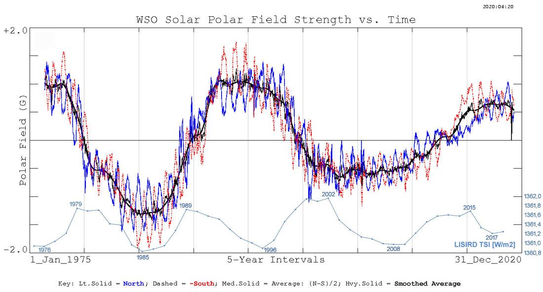
Figure 5: The amplitude of the poloidal magnetic field is largest during the years around the TSI minima; the field changes polarity during the TSI maxima (source: WSO³⁷). The blue and red graphs represent the activity of the magnetic north pole and inverted south pole, respectively; the black graph represents the average magnetic activity (the thick line represents the smoothed average). The LISIRD TSI is shown in light blue color at the bottom.

---

Method

The Excel data file describes for the period 1880-2019 the LISIRD TSI dataset and the HadSST3 dataset + all correlations (based on Pearson correlation coefficient) and explained variances (based on R² method via linear regression) listed in figures 1 through 4. The data shown in the figures is processed in the Excel data file as follows:

• Figure 1: LISIRD TSI (column C), HadSST3 (column D); columns I to AW show data + correlations with regard to the periods 1880-2018 and 1880-1985 for: the maxima, primary maxima, secondary maxima, minima, primary minima & secondary minima.

• Figure 2: Temperature profile Hale cycle (column CW), temperature profile Schwabe cycle (column CX); columns BB to CS present the underlying calculation method for the Hale cycle temperature profile. The trend has been removed from each of the 4 reference profiles based on a slope corresponding to a temperature increase of 0,0028 C per year (= 0,28 °C per 100 years); a higher or lower value means that the second primary minimum in figure 2 does not end exactly at zero. The Hale cycle temperature profile is composed of 4 series of data around the TSI minima and maxima years, whereby the profile of the primary minima years is split into 2 parts (column BX and column CN therefore contain the same data). Only the values labeled with a * are included in the Hale cycle temperature profile. The Schwabe cycle temperature profile has been derived directly from the Hale cycle temperature profile.

• Figure 3: [TOP] LISIRD (column DY), HadSST3 (column DZ); [BOTTOM] LISIRD with corrected secondary minima (column EG), HadSST3 (column EH). The correction value is the lowest value, for which the average correlation value of the primary and secondary data is found for the combination.

• Figure 4: 1-year mean corrected LISIRD (column FH), HadSST3 (column FI); 3-year mean corrected LISIRD (column GG), HadSST3 (column GH); 5-year mean corrected LISIRD (column HF), HadSST3 (column HG); 7-year mean corrected LISIRD (IE column), HadSST3 (IF column); 9-year mean corrected LISIRD (column JD), HadSST3 (column JE); 11-year mean corrected LISIRD (column KC), HadSST3 (column KD). The correction value represents the lowest value for each minimum period whereby for the minima combination the average correlation value of the primary and secondary data is found.

Download: Excel data file

---

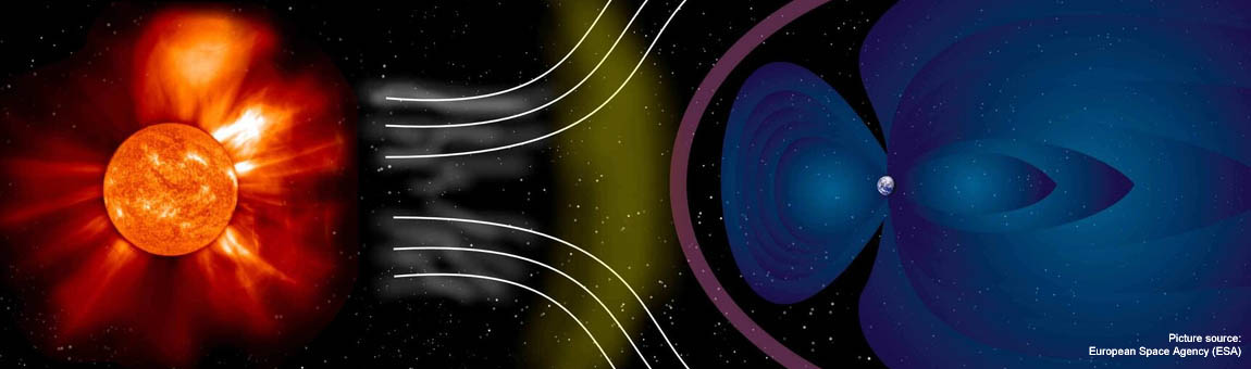
Figure A: The magnetic field of the sun & the magnetic field of the Earth.

---

---

References:

1. de Jager, C., Versteegh G.J.M. & van Dorland, R. Climate Change Scientific Assessment and Policy Analysis - Scientific Assessment of Solar Induced Climate Change, Rapport KNMI & NIOZ, 14 (2006).
2. Smith, T.M. & Reynolds, R.W. Extended Reconstruction of Global Sea Surface Temperatures Based on COADS Data (1854-1997), J. Clim., 16, 1495-1510 (2003).
3. Cheng, L., Zhu, J., Abraham, J., Trenberth, K.E., Fasullo, J.T., Zhang, B., Yu, F., Wan, L., Chen, X. & Song, X. 2018 Continues Record Global Ocean Warming, Adv. Atmos. Sci., 36, 249-252 (2019).
4. Camp, C.D. & Tung, K.K. Surface warming by the solar cycle as revealed by the composite mean difference projection, Geophys. Res. Lett., 1-5 (2007).
5. Shavif, N.J. The Role of the Solar Forcing in the 20th century climate change, International Seminar on Nuclear War and Planetary Emergencies, 44, 279-286 (2012).
6. Shavif, N.J. On climate response to changes in the cosmic ray flux and radiative budget, J. Geophys. Res, 110, A08105 (2005).
7. Scafetta, N. Discussion on common errors in analyzing sea level accelerations, solar trends and global warming, Pattern Recogn. Phys., 1, 37-57 (2013).
8. Solanki, S.K., Krivova, N.A. & Haigh, J.D. Solar Irradiance Variability and Climate, Annu. Rev. Astron. Astrophys., 51, 311-351 (2013).
9. Scafetta, N., Willson, R.C., Lee, J.N. & R.C. Wu, D.L. Modeling Quiet Solar Luminosity Variability from TSI Satellite Measurements and Proxy Models during 1980-2018, Remote Sens., 11 (21), 2569 (1-27), (2019).
10. Lean, J., Beer, J. & Bradley, R. Reconstruction of solar irradiance since 1610: Implications for climate change, Geophys. Res. Lett., 22 (23), 3195-3198 (1995).
11. Hoyt, D.V., & Schatten, K.H. A Discussion of Plausible Solar Irradiance Variations, 1700-1992, J. Geophys. Res., 98 (A11), 18,895-18,906 (1993).
12. Hale, G.E. On the probable existence of a magnetic field in sun-spots, ApJ, 28, 315-343 (1908)
13. Zolotova, N.V. & Ponyavin, D.I. The Gnevyshev-Ohl Rule and Its Violations, geomagn aeronomy+, 55 (7), 902-906 (2015).
14. IPCC, 2013: Climate Change 2013: The Physical Science Basis. Contribution of Working Group I to the Fifth Assessment Report of the Intergovernmental Panel on Climate Change [Stocker, T.F., D. Qin, G.-K. Plattner, M. Tignor, S.K. Allen, J. Boschung, A. Nauels, Y. Xia, V. Bex and P.M. Midgley (eds.)]. Cambridge University Press, Cambridge, United Kingdom and New York, NY, USA, 1535 pp. (2013). Quote page 56 (Technical Summary): "Longer term forcing is typically estimated by comparison of solar minima (during which variability is least)." Quote page 689 (Chapter 8): "The year 1750, which is used as the preindustrial reference for estimating RF, corresponds to a maximum of the 11-year SC. Trend analysis are usually performed over the minima of the solar cycles that are more stable. For such trend estimates, it is then better to use the closest SC minimum, which is in 1745. ... Maxima to maxima RF give a higher estimate than minima to minima RF, but the latter is more relevant for changes in solar activity."
15. Hiyahara, H., Yokoyama, Y. & Masude, K. Possible link between multi-decadal climate cycles and periodic reversals of solar magnetic field polarity, Earth Planet. Sci. Lett., 272, 290-295 (2008).
16. Lasp Interactive Solar Irradiance Datacenter: Historical Total Solar Irradiance Reconstruction, Time Series, author: Greg Kopp
17. Kopp, G., Krivova, N., Wu, C.J. & Lean, J. The Impact of the Revised Sunspot Record on Solar Irradiance Reconstructions, Sol. Phys., 291, 2951-2965 (2016).
18. Dudok de Wit, T., Kopp, G., Frölich, C. & Schöll, M. Methodology to create a new total solar irradiance record: Making a composite out of multiple data records, Geophys. Res. Lett., 44 (3), 1196-1203 (2017).
19. Met Office Hadley Centre observations datasets: HadSST3.1.1.0 Data [annual globe] (2019).
20. Narsimha, R. & Bhattacharyya, S. A wavelet cross-spectral analysis of solar-ENSO-rainfall connections in the Indian monsoons, Appl. Comput. Harmon. Anal., 28, 285-295 (2010).
21. Gnevyshev, M.N. Essential features of the 11-year solar cycle, Sol. Phys., 51, 175-183 (1977).
22. Svensmark, H. Cosmic rays, clouds and climate, Europhys. News, 46 (2), 26-29 (2015).
23. Stott, P.A., Jones, G.S. & Mitchell, J.F.B. Do Models Underestimate the Solar Contribution to Recent Climate Change?, J. Clim., 16, 4079-4093 (2003).
24. Haigh, J.D. The Sun and the Earth's Climate, Living Rev. Sol. Phys., 46 (2), 26-29 (2007).
25. Ziskin, S. & Shavif, N.J. Quantifying the role of solar radiative forcing over the 20th century, Adv. Space Res., 50, 762-2776 (2012).
26. Holmes, R.I. Thermal Enhancement on Planetary Bodies and the Relevance of the Molar Mass Version of the Ideal Gas Law to the Null Hypothesis of Climate Change, Earth Sciences., 7 (3), 107-123 (2018).
27. Shavif, N.J. Using the oceans as a calorimeter to quantify the solar radiative forcing, J. Geophys. Res. Solid Earth, 113 (2008).
28. Scafetta, N. & West, B.J. Estimated solar contribution to the global surface warming using the ACRIM TSI satellite composite, Geophys. Res. Lett., 32, L18713: 1-4 (2005).
29. PAGES 2k Consortium Consistent multi-decadal variability in global temperature reconstructions and simulations over the Common Era (Supplementary Materials), Nat Geosci., 12 (8), 643-649 (2019).
30. Usoskin, I.G., Solanki, S.K. & Kovaltsov, G.A. Grand minima and maxima of solar activity: new observational constraints, Astron. Astrophys., 471, 301-309 (2007).
31. Karof, C. & Svensmark, H. How did the Sun affect the climate when life evolved on the Earth? - A case study on the young solar twin κ¹ Ceti, Astron. Astrophys., 471, 301-309 (2007).
32. Scafetta, N. & West, B.J. Is climate sensitive to solar variability?, Phys. Today, 61 (3), 50-51 (2008).
33. Coddington, O., Lean, J.L., Pilewskie, P., Snow, M. & Lindholm, D. A solar irradiance climate data record, Bull. Amer. Meteor., 1265-1282 (2016).
34. Feynmann, J. & Ruzmaikin, A. The Centennial Gleissberg Cycle and its association with extended minima, J. Geophys. Res. Space Physics, 19, 6027-6041 (2014).
35. Jose, P.D. Sun's motion and sunspots, Astron. J., 70 (3), 193-200 (1965).
36. Usoskin, I.G., Galler, Y., Lopes, F., Kovaltsov, G.A. & Hulot, G. Solar activity during the Holocene: the Hallstatt cycle and its consequence for grand minima and maxima, Astron. Astrophys., 587, A150: 1-10 (2016).
37. The Wilcox Solar Observatory: Solar Polar Field Strength [.gif] (2020).